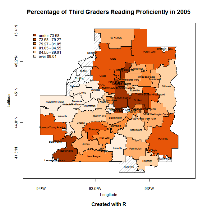
I decided to make a more advanced map, one with some relevance to my graduate studies in evaluation and educational psychology. This map shows geographic variation in third grade reading proficiency as measured by the 2005 Minnesota Comprehensive Assessment (MCA). Click on the thumbnail to enlarge:
Merging test scores to the attribute data frame was difficult. The attribute data frame must evidently remain sorted in the same order in which it was converted to an sp class object. I found this out after merging district test scores to the attribute data frame and finding that Cannon Falls had migrated up to Minneapolis. I created a row number variable to re-sort the data frame back to its original order before adding it back to the sp object. I’m betting there is a better way to achieve the same type of join. In the future, I will probably join additional variables to the DBF portion of the SHP file before calling it into R.
Here is the script:
library(maptools)

library(rgdal)

library(RColorBrewer)

library(classInt)
#get data
mca05r3m <- read.table(file.choose()) #MCA scores from MDE
districts <- readShapePoly(file.choose(), proj4string=CRS("+proj=utm +zone=15 +ellps=GRS80 +datum=NAD83")) #school districts from MetroGIS
#prepare data
districts <- spTransform(districts, CRS=CRS("+proj=longlat"))
districts@data$row <- as.numeric(row.names(districts@data)) #necessary for linking attributes back to polygons after merge
mca05r3m$proficient <- with(mca05r3m, percentLevel3 + percentLevel4 + percentLevel5) #MCA levels 3-5 represent proficiency
temp <- merge(districts@data, mca05r3m, by="SD_NUMBER", all.x=T, sort=F) #merge scores to attribute data frame
districts@data <- temp[order(temp$row),] #order is key
districts@data
#set up the choropleth with helpful code from GeogR
plotvar <- districts@data$proficient
nclr <- 6
plotclr <- brewer.pal(nclr,"Oranges")
plotclr <- plotclr[nclr:1] #reordering colors looks better
class <- classIntervals(plotvar, nclr, style="quantile")
colcode <- findColours(class, plotclr, digits=4)
colcode
#map it
plot(districts, density=16, col="grey", axes=T, cex.axis=.75) #hatches missing data
plot(districts, col=colcode, add=T)
text(coordinates(districts), labels=districts$SD_NAME.x, cex=.5)
title(main="Percentage of Third Graders Reading Proficiently in 2005", sub="Created with R",font.sub=2)
title(xlab="Longitude",ylab='Latitude',cex.lab=.75,line=2.25)
legend(-94.1, 45.4, legend=names(attr(colcode, "table")), fill=attr(colcode, "palette"), cex=0.75, bty="n")
Sources of data and code include:
http://education.state.mn.us/
http://www.metrogis.org/
http://geography.uoregon.edu/GeogR/index.html