EvaluationDashboard.com

Applying generalizability theory with R

Posted on October 10, 2012 by canoemoore

One of the things I like about my current job is getting to apply generalizability theory. I have to confess that I didn’t appreciate G theory at first, but now that I’m analyzing data from performance assessments (i.e., ratings of instructional effectiveness) I think it’s great for a number of reasons. I like the concept of universe scores, treating items as a random facet, estimating multiple sources of error, the ability to focus on different objects of measurement (e.g., ratees and raters), and G theory’s strong emphasis on finding ways to increase generalizability (i.e., decision studies). And as someone who has far more experience with item response theory (IRT) where conditional standard errors of measurement (CSEMs) are the norm, I’m especially intrigued by the prospect of using G theory to estimate CSEMs.

It’s pretty obvious from this blog that I like statistical programming with because it helps me learn methods far better than simply reading about them or using a pre-existing software package. In that vein, I decided to write some functions to conduct G and D studies with . I’ve been using synthetic data from Brennan’s book and Shavelson and Webb’s book to ensure that my results match theirs. The nice thing about using for G theory is that you can choose functions for many different packages to fully apply G theory. For example, by using lme4 to estimate variance components, arm to extract standard errors of random intercepts, and ggplot2 to create faceted plots, I am able to create “vertical ruler” plots, which are prevalent among practitioners of many-facets Rasch. Such plots make it easy to identify the (statistically significantly) highest and lowest performers as well as the most lenient and stringent raters.

The plots below illustrate how I’ve been implementing G theory with . The plots were produced from Brennan’s synthetic data set number 4, and the dependability coefficients match those from GENOVA. I’ve never developed an package, but given that no one else has so far, I’d be interested in doing so with the code I’m developing.

Posted in Praxes | 1 Comment

Estimating congeneric reliability with R

Posted on September 22, 2012 by canoemoore

I was recently tasked with estimating the reliability of scores composed of items on different scales. The lack of a common scale could be seen in widely varying item score means and variances. As discussed by Graham, it’s not widely known in applied educational research that Cronbach’s alpha assumes essential tau-equivalence and underestimates reliability when the assumption isn’t met. A friend made a good suggestion to consider stratified alpha, which is commonly used to estimate internal consistency when scores are composed of multiple choice items (scored 0-1) and constructed response items (e.g., scored 0-4). However, the assessment with which I was concerned does not have clear item-type strata. I decided to estimate congeneric reliability because it makes few assumptions (e.g., unidimensionality) and doesn’t require grouping items into essentially tau-equivalent strata.

With the help of Graham’s paper and a LISREL tutorial by Raykov I wrote an program that estimates congeneric reliability. The program uses Fox’s sem() library to conduct the confirmatory factor analysis with minimal constraints (variance of common true score fixed at 1 for identifiability). The estimated loadings and error variances are then summed to calculate reliability (i.e., the ratio of true score variance to observed score variance) as:

$hat{rho}_{XX'} = frac { left( sum hat{lambda}_i right) ^ 2} {left( sum hat{lambda}_i right) ^ 2 + sum hat{delta}_{i} }$ .

I obtained a congeneric reliability estimate of 0.80 and an internal consistency estimate of 0.58 for the scores I was analyzing. If the items had been essentially tau-equivalent, then the reliability estimates would have been the same. If I had assumed tau-equivalence, than I would have underestimated the reliability of the total scores (and overestimated standard errors of measurement). The example below replicates Graham’s heuristic example.

> ############################################
> #Replicate results from Graham (2006) to check congeneric reliability code/calculations.
>
> library(sem)
> library(psych)
> library(stringr)
>
> #Variance/covariance matrix
> S.graham <- readMoments(diag = T, names = paste("x", 1:7, sep = ""))
1:  4.98
2:  4.60  5.59
4:  4.45  4.42  6.30
7:  3.84  3.81  3.66  6.44
11:  5.71  5.67  5.52  4.91 11.86
16: 23.85 23.68 22.92 19.87 34.28 127.65
22: 46.53 46.20 44.67 38.57 62.30 244.36 471.95
29:
Read 28 items
>
> ############################################
> #A function to estimate and compare congeneric reliability and internal consistency
> funk.congeneric <- function(cfa.out) {
+   names.loadings <- str_detect(names(cfa.out$coeff), "loading")
+   names.errors <- str_detect(names(cfa.out$coeff), "error")
+   r.congeneric <- sum(cfa.out$coeff[names.loadings]) ^ 2 /
+     (sum(cfa.out$coeff[names.loadings]) ^ 2 + sum(cfa.out$coeff[names.errors]))
+   round(c("Congeneric" = r.congeneric, "Alpha" = alpha(cfa.out$S)$total$raw_alpha), 2)
+ }
>
> ############################################
> #Congeneric model; tau-equivalent items
> model.graham <- specifyModel()
1: T -> x1, loading1
2: T -> x2, loading2
3: T -> x3, loading3
4: T -> x4, loading4
5: T -> x5, loading5
6: x1 <-> x1, error1
7: x2 <-> x2, error2
8: x3 <-> x3, error3
9: x4 <-> x4, error4
10: x5 <-> x5, error5
11: T <-> T, NA, 1
12:
Read 11 records
> cfa.out <- sem(model = model.graham, S = S.graham, N = 60)
> summary(cfa.out)
Model Chisquare =  0.11781   Df =  5 Pr(>Chisq) = 0.99976
Chisquare (null model) =  232.13   Df =  10
Goodness-of-fit index =  0.9992
Adjusted goodness-of-fit index =  0.99761
RMSEA index =  0   90% CI: (NA, NA)
Bentler-Bonnett NFI =  0.99949
Tucker-Lewis NNFI =  1.044
Bentler CFI =  1
SRMR =  0.0049092
AIC =  20.118
AICc =  4.6076
BIC =  41.061
CAIC =  -25.354
Normalized Residuals
Min.   1st Qu.    Median      Mean   3rd Qu.      Max.
-0.038700 -0.008860 -0.000002  0.004700  0.002450  0.119000
R-square for Endogenous Variables
x1     x2     x3     x4     x5
0.9286 0.8175 0.6790 0.4962 0.5968
Parameter Estimates
Estimate Std Error z value Pr(>|z|)
loading1 2.15045  0.21595   9.9580  2.3263e-23 x1 <--- T
loading2 2.13776  0.24000   8.9073  5.2277e-19 x2 <--- T
loading3 2.06828  0.26941   7.6770  1.6281e-14 x3 <--- T
loading4 1.78754  0.29136   6.1352  8.5040e-10 x4 <--- T
loading5 2.66040  0.38141   6.9752  3.0535e-12 x5 <--- T
error1   0.35559  0.17469   2.0356  4.1793e-02 x1 <--> x1
error2   1.02000  0.25339   4.0255  5.6861e-05 x2 <--> x2
error3   2.02222  0.41688   4.8509  1.2293e-06 x3 <--> x3
error4   3.24471  0.62679   5.1767  2.2583e-07 x4 <--> x4
error5   4.78227  0.94911   5.0387  4.6871e-07 x5 <--> x5
Iterations =  21
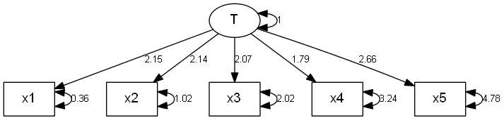
> pathDiagram(cfa.out, edge.labels = "values", ignore.double = F, rank.direction = "TB")

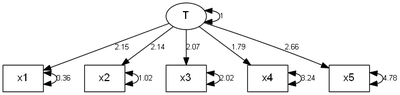
> funk.congeneric(cfa.out)
Congeneric      Alpha
0.91       0.91
>
> ############################################
> #Congeneric model; tau-inequivalent items
> model.graham <- specifyModel()
1: T -> x1, loading1
2: T -> x2, loading2
3: T -> x3, loading3
4: T -> x4, loading4
5: T -> x7, loading7
6: x1 <-> x1, error1
7: x2 <-> x2, error2
8: x3 <-> x3, error3
9: x4 <-> x4, error4
10: x7 <-> x7, error7
11: T <-> T, NA, 1
12:
Read 11 records
> cfa.out <- sem(model = model.graham, S = S.graham, N = 60)
> summary(cfa.out)
Model Chisquare =  0.0072298   Df =  5 Pr(>Chisq) = 1
Chisquare (null model) =  353.42   Df =  10
Goodness-of-fit index =  0.99995
Adjusted goodness-of-fit index =  0.99985
RMSEA index =  0   90% CI: (NA, NA)
Bentler-Bonnett NFI =  0.99998
Tucker-Lewis NNFI =  1.0291
Bentler CFI =  1
SRMR =  0.0010915
AIC =  20.007
AICc =  4.497
BIC =  40.951
CAIC =  -25.464
Normalized Residuals
Min.   1st Qu.    Median      Mean   3rd Qu.      Max.
-2.76e-02 -1.27e-04 -1.00e-07 -1.92e-03  1.96e-04  3.70e-03
R-square for Endogenous Variables
x1     x2     x3     x4     x7
0.9303 0.8171 0.6778 0.4942 0.9902
Parameter Estimates
Estimate Std Error z value  Pr(>|z|)
loading1  2.15247 0.212984  10.10624 5.1835e-24 x1 <--- T
loading2  2.13719 0.237279   9.00711 2.1156e-19 x2 <--- T
loading3  2.06646 0.266419   7.75646 8.7336e-15 x3 <--- T
loading4  1.78392 0.287599   6.20279 5.5470e-10 x4 <--- T
loading7 21.61720 2.015041  10.72792 7.5272e-27 x7 <--- T
error1    0.34688 0.090227   3.84451 1.2080e-04 x1 <--> x1
error2    1.02240 0.200635   5.09584 3.4720e-07 x2 <--> x2
error3    2.02973 0.382466   5.30694 1.1148e-07 x3 <--> x3
error4    3.25764 0.605376   5.38118 7.3998e-08 x4 <--> x4
error7    4.64661 6.387765   0.72742 4.6697e-01 x7 <--> x7
Iterations =  38
> pathDiagram(cfa.out, edge.labels = "values", ignore.double = F, rank.direction = "TB")

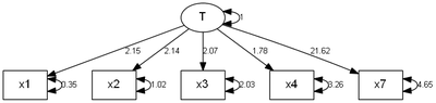
> funk.congeneric(cfa.out)
Congeneric      Alpha
0.99       0.56

Posted in Praxes | 1 Comment

Converting Rasch units (RITs) to thetas

Posted on May 25, 2012 by canoemoore

How do you place Measures of Academic Progress (MAP) Rash unit scores (RITs) on the normal theta metric (and vice versa)? I searched the Web but couldn’t find a straightforward answer. What I’ve gathered from various sources is that RIT scores are just logits multiplied by 10 and centered on 200. From there, logits can be transformed to thetas based on the probabilities of the respective distributions, as shown in the code below.

RIT scores are new to me because I’ve worked mostly with the 3-parameter model until recently. I’ve noticed that a lot psychometricians who use item response theory (IRT) fall into one of two camps: Rasch or 3PL. My personal preference is somewhere in the middle. I think 1) it’s unrealistic to assume items discriminate equally and 2) estimates of a are useful for test construction and adaptive selection. The c parameter, on the other hand, is costly to estimate and not entirely essential. So I guess you could say I’m a dispassionate 2PL guy.

> #Simulate some thetas (z-scores).
> thetas <- sort(rnorm(20))
> thetas
[1] -1.34485345 -1.08206871 -1.04673807 -0.98990444
[5] -0.96802821 -0.81766629 -0.56671883 -0.18795885
[9] -0.17779446 -0.08314090 -0.04615256  0.13611619
[13]  0.13796440  0.43172163  0.47472683  0.57965345
[17]  0.64315758  0.71571489  1.10205842  1.16067809
>
> #Convert thetas to probabilities then logits.
> p <- pnorm(thetas)
> logits <- log(p / (1 - p))
>
> #Convert logits to RITs.
> RITs <- logits * 10 + 200
> RITs
[1] 176.7823 181.8148 182.4653 183.5001 183.8947 186.5552
[7] 190.8243 196.9958 197.1587 198.6728 199.2634 202.1739
[13] 202.2035 206.9477 207.6533 209.3914 210.4565 211.6874
[19] 218.5559 219.6538
>
> #Place RITs on normal theta metric.
> funk.RITs.thetas <- function(x) {
+   qnorm(plogis((x - 200) / 10))
+ }
> funk.RITs.thetas(RITs)
[1] -1.34485345 -1.08206871 -1.04673807 -0.98990444
[5] -0.96802821 -0.81766629 -0.56671883 -0.18795885
[9] -0.17779446 -0.08314090 -0.04615256  0.13611619
[13]  0.13796440  0.43172163  0.47472683  0.57965345
[17]  0.64315758  0.71571489  1.10205842  1.16067809

Posted in Praxes | Comments Off

Urban canoeing: Dining at The Sample Room

Posted on October 22, 2011 by canoemoore

I finally found some time to upgrade my Wike canoe trailer. As I mentioned in an earlier post, the trailer had a hard time handling Scrappy, my 17′ Alumacraft canoe. I added a U-bolt to adequately secure the bow, and I reinforced the aluminum axle with an iron rod to keep it from bending. It’s working well enough to resume canoeing around Minneapolis without a car shuttle.

Amy and I took the trailer down Saint Anthony Parkway to the Mississippi River for some paddling at dusk. We put in at the Camden Railroad Bridge. The moon was huge, so we had no trouble navigating after the sun went down. You can see the moon above Psycho Suzi’s Motor Lounge in the picture below.

We got hungry on the river, so we stopped at one of our favorite spots in Northeast: The Sample Room. The restaurant conveniently has its own dock and stairway up the steep bank of the river. Our server even comped us a drink for canoeing in with our life jackets! After dining on the patio, we continued down the Mississippi to Boom Island Park and rode our bikes home from there. It was a fun way to spend an evening in Minneapolis!

Posted in Personal | Comments Off

Urban canoeing: North/Northeast Minneapolis

Posted on September 11, 2011 by canoemoore

Back in July, my friend, Joe, and I were laid off during the state government shutdown. It was a stressful time, not knowing if or how the shutdown would end and having to cut back on expenses to make up for lost income. We decided to put our worries behind us for a day and make the most of our time off by taking a canoe trip down the Mississippi River.

We started under a rainy sky in North Minneapolis, at the Camden Avenue bridge boat launch. I had never paddled the northern section of the Mississippi as it passes through Minneapolis. It’s an industrial stretch of river, but plans have been developed to transform it into a more attractive and accessible destination, much like the river’s character further downstream.

A highlight of our trip occurred just above the uppermost lock on the Mississippi River, near Saint Anthony Falls. As we explored the northern channel around Nicollet Island, we paddled past a ceremony honoring the ratifications of an Urban Conservation Treaty for Migratory Birds attended by Mayor R.T. Rybak and several other environmental enthusiasts. A local news station filmed us paddling by to highlight the outdoor recreation potential of urban rivers and the importance of conserving them. Check out my sweet J-strokes!

The City of Minneapolis recently held a design competition for the stretch “Above the Falls.” The video accompanying the winning proposal is below. As a resident of Northeast Minneapolis (river left), it’s thrilling to envision an inviting riverfront right in my neighborhood.