My last post described how test development designs could be thought of as multistage sampling designs and how multilevel Rasch could be used to estimate parameters under that assumption. I decided to use ![]() to compare estimates from the usual Rasch model, the generalized linear model (GLM) with a logit link, and generalized linear mixed-effects regression (GLMER), treating items as fixed then random effects. The GLMER model with item fixed effects exhibited the best fit of the Law School Admission Test (LSAT) data provided with the
to compare estimates from the usual Rasch model, the generalized linear model (GLM) with a logit link, and generalized linear mixed-effects regression (GLMER), treating items as fixed then random effects. The GLMER model with item fixed effects exhibited the best fit of the Law School Admission Test (LSAT) data provided with the ltm package. Moreover, intraclass correlation has reduced the effective sample size relative to simple random sampling, lending further support to the multilevel Rasch approach.
#Load libraries.

library(ltm)

library(lme4)

library(xtable)
#Prepare data for GLM.
LSAT.long <- reshape(LSAT, times=1:5, timevar="Item", varying=list(1:5), direction="long")
names(LSAT.long) <- c("Item", "Score", "ID")
LSAT.long$Item <- as.factor(LSAT.long$Item)
LSAT.long$ID <- as.factor(LSAT.long$ID)
#Compute Rasch, GLM, and GLMER estimates and compare fit.
out.rasch <- rasch(LSAT, constraint=cbind(ncol(LSAT)+1, 1))
print(xtable(summary(out.rasch)$coefficients, digits=3), type="html")
| value | std.err | z.vals | |
|---|---|---|---|
| Dffclt.Item1 | -2.872 | 0.129 | -22.307 |
| Dffclt.Item2 | -1.063 | 0.082 | -12.946 |
| Dffclt.Item3 | -0.258 | 0.077 | -3.363 |
| Dffclt.Item4 | -1.388 | 0.086 | -16.048 |
| Dffclt.Item5 | -2.219 | 0.105 | -21.166 |
| Dscrmn | 1.000 |
out.glm <- glm(Score ~ Item, LSAT.long, family="binomial")

print(xtable(summary(out.glm)$coefficients, digits=3), type="html")
| Estimate | Std. Error | z value | Pr(> |z|) | |
|---|---|---|---|---|
| (Intercept) | 2.498 | 0.119 | 20.933 | 0.000 |
| Item2 | -1.607 | 0.138 | -11.635 | 0.000 |
| Item3 | -2.285 | 0.135 | -16.899 | 0.000 |
| Item4 | -1.329 | 0.141 | -9.450 | 0.000 |
| Item5 | -0.597 | 0.152 | -3.930 | 0.000 |
out.glmer <- glmer(Score ~ Item + (1|ID), LSAT.long, family="binomial")

print(xtable(summary(out.glmer)@coefs, digits=3, caption="Fixed effects"), type="html", caption.placement="top")

print(xtable(summary(out.glmer)@REmat, digits=3, caption="Random effects"), type="html", caption.placement="top", include.rownames=F)
| Estimate | Std. Error | z value | Pr(> |z|) | |
|---|---|---|---|---|
| (Intercept) | 2.705 | 0.129 | 21.029 | 0.000 |
| Item2 | -1.711 | 0.145 | -11.774 | 0.000 |
| Item3 | -2.467 | 0.142 | -17.353 | 0.000 |
| Item4 | -1.406 | 0.148 | -9.498 | 0.000 |
| Item5 | -0.623 | 0.160 | -3.880 | 0.000 |
| Groups | Name | Variance | Std.Dev. |
|---|---|---|---|
| ID | (Intercept) | 0.502 | 0.70852 |
out.glmer.re <- glmer(Score ~ (1|Item) + (1|ID), LSAT.long, family="binomial")

print(xtable(summary(out.glmer.re)@coefs, digits=3, caption="Fixed effects"), type="html", caption.placement="top")

print(xtable(summary(out.glmer.re)@REmat[,-6], digits=3, caption="Random effects"), type="html", caption.placement="top", include.rownames=F)
| Estimate | Std. Error | z value | Pr(> |z|) | |
|---|---|---|---|---|
| (Intercept) | 1.448 | 0.379 | 3.818 | 0.000 |
| Groups | Name | Variance | Std.Dev. |
|---|---|---|---|
| ID | (Intercept) | 0.45193 | 0.67226 |
| Item | (Intercept) | 0.70968 | 0.84243 |
print(xtable(AICs.Rasch.GLM <- data.frame(Rasch=summary(out.rasch)$AIC, GLM=summary(out.glm)$aic, GLMER.fe=summary(out.glmer)@AICtab$AIC, GLMER.re=summary(out.glmer.re)@AICtab$AIC, row.names="AIC"), caption="Akaike's information criteria (AICs)"), type="html", caption.placement="top")
| Rasch | GLM | GLMER.fe | GLMER.re | |
|---|---|---|---|---|
| AIC | 4956.11 | 4996.87 | 4950.80 | 4977.25 |
#Easiness estimates.

easiness <- data.frame(Rasch=out.rasch$coefficients[,1],

GLM=c(out.glm$coefficients[1], out.glm$coefficients[1]+out.glm$coefficients[-1]),

GLMER.fe=c(fixef(out.glmer)[1], fixef(out.glmer)[1]+fixef(out.glmer)[-1]),

GLMER.re=fixef(out.glmer.re)+unlist(ranef(out.glmer.re)$Item))

print(xtable(easiness, digits=3), type="html")
| Rasch | GLM | GLMER.fe | GLMER.re | |
|---|---|---|---|---|
| Item 1 | 2.872 | 2.498 | 2.705 | 2.527 |
| Item 2 | 1.063 | 0.891 | 0.994 | 0.917 |
| Item 3 | 0.258 | 0.213 | 0.237 | 0.224 |
| Item 4 | 1.388 | 1.169 | 1.299 | 1.201 |
| Item 5 | 2.219 | 1.901 | 2.082 | 1.938 |
#Estimated probabilities of a correct response.

pr.correct <- sapply(easiness, plogis)

row.names(pr.correct) <- row.names(easiness)

print(xtable(pr.correct, digits=3), type="html")
| Rasch | GLM | GLMER.fe | GLMER.re | |
|---|---|---|---|---|
| Item 1 | 0.946 | 0.924 | 0.937 | 0.926 |
| Item 2 | 0.743 | 0.709 | 0.730 | 0.714 |
| Item 3 | 0.564 | 0.553 | 0.559 | 0.556 |
| Item 4 | 0.800 | 0.763 | 0.786 | 0.769 |
| Item 5 | 0.902 | 0.870 | 0.889 | 0.874 |
#Difficulty estimates.

difficulties <- easiness*-1

print(xtable(difficulties, digits=3), type="html")
| Rasch | GLM | GLMER.fe | GLMER.re | |
|---|---|---|---|---|
| Item 1 | -2.872 | -2.498 | -2.705 | -2.527 |
| Item 2 | -1.063 | -0.891 | -0.994 | -0.917 |
| Item 3 | -0.258 | -0.213 | -0.237 | -0.224 |
| Item 4 | -1.388 | -1.169 | -1.299 | -1.201 |
| Item 5 | -2.219 | -1.901 | -2.082 | -1.938 |
#Calculate design effects and effective samples sizes from intraclass correlation coefficients and sampling unit sizes.

multistage.consequences <- function(ICC, N) {

M <- nrow(LSAT.long)

n <- M/N #number of responses per item

deff <- 1+(n-1)*ICC

M.effective <- trunc(M/deff)

return(data.frame(ICC, M, N, n, deff, M.effective))

}

model.ICC.Item <- glmer(Score ~ 1 + (1|Item), family=binomial, data=LSAT.long)

ICC.Item <- as.numeric(VarCorr(model.ICC.Item)$Item)/(as.numeric(VarCorr(model.ICC.Item)$Item)+pi^2/3)

multistage.Item <- multistage.consequences(ICC.Item, 5)

model.ICC.ID <- glmer(Score ~ 1 + (1|ID), family=binomial, data=LSAT.long)

ICC.ID <- as.numeric(VarCorr(model.ICC.ID)$ID)/(as.numeric(VarCorr(model.ICC.ID)$ID)+pi^2/3)

multistage.ID <- multistage.consequences(ICC.ID, 1000)

multistage <- data.frame(cbind(t(multistage.Item), t(multistage.ID)))

names(multistage) <- c("Item", "ID")

print(xtable(multistage, digits=3), type="html")
| Item | ID | |
|---|---|---|
| ICC | 0.159 | 0.070 |
| M | 5000.000 | 5000.000 |
| N | 5.000 | 1000.000 |
| n | 1000.000 | 5.000 |
| deff | 160.295 | 1.281 |
| M.effective | 31.000 | 3903.000 |
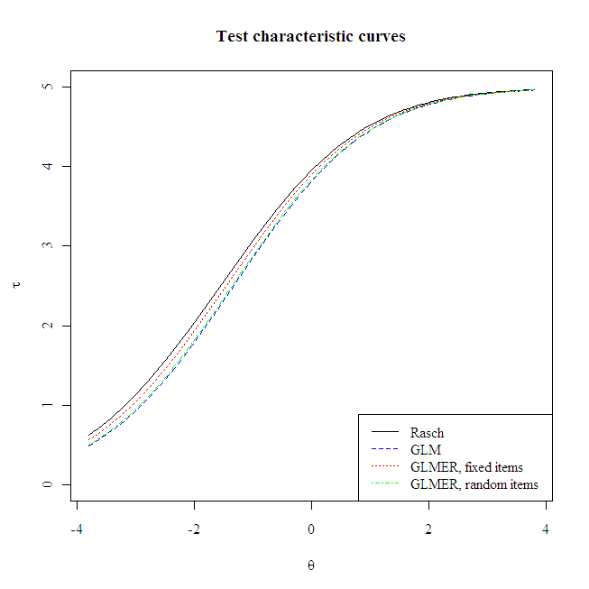
#Plot test characteristic curves

plot.tcc <- function(difficulties, add, col, lty) {

thetas <- seq(-3.8,3.8,length=100)

temp <- matrix(nrow=length(difficulties), ncol=length(thetas))

for(i in 1:length(thetas)) {for(theta in thetas) temp[,which(thetas==theta)] <- plogis(theta-difficulties)}

if(missing(add)) {plot(thetas, colSums(temp), ylim=c(0,5), col=NULL, ylab=expression(tau), xlab=expression(theta), main="Test characteristic curves")}

lines(thetas, colSums(temp), col=col, lty=lty)

}

plot.tcc(difficulties=difficulties[,1], col="black", lty=1)

plot.tcc(difficulties=difficulties[,2], add=T, col="blue", lty=2)

plot.tcc(difficulties=difficulties[,3], add=T, col="red", lty=3)

plot.tcc(difficulties=difficulties[,4], add=T, col="green", lty=4)

legend("bottomright", c("Rasch", "GLM", "GLMER, fixed items", "GLMER, random items  "), col=c("black", "blue", "red", "green"), lty=1:4)