
My job as a Quantitative Analyst at the Minnesota Department of Education requires me to “provide evaluation, statistical, and psychometric support to the Division of Research and Assessment through the entire process of design, development, and reporting to the Minnesota assessment system.” That’s an accurate job description, but a little vague. What I really do is write a lot of ![]() code to apply item response theory (IRT) and compare item and test characteristics across multiple years and/or forms to maintain high quality.
code to apply item response theory (IRT) and compare item and test characteristics across multiple years and/or forms to maintain high quality.
![]() is great for plotting item and test characteristics across multiple years and/or forms, but it requires using a few packages in concert (i.e., to my knowledge there is no single package designed for this purpose). The irtoys package provides many useful functions for test development under IRT; the plyr package allows one to apply irtoys’ functions to subsets of item parameters in a data set (e.g., by strand); and the ggplot2 package allows one to overlay and facet item and test curves.
is great for plotting item and test characteristics across multiple years and/or forms, but it requires using a few packages in concert (i.e., to my knowledge there is no single package designed for this purpose). The irtoys package provides many useful functions for test development under IRT; the plyr package allows one to apply irtoys’ functions to subsets of item parameters in a data set (e.g., by strand); and the ggplot2 package allows one to overlay and facet item and test curves.
In the following reproducible example, I graphically compare item and test characteristics of the 2009 and 2010 grade 3 Minnesota Comprehensive Assessments of reading ability. Note that for simplicity, I have excluded two polytomous items from 2009 and a few dichotomous items from 2010 from the published item parameter estimates. Also note that items have been assigned to strands arbitrarily in this example. Graphs such as these allow us to answer questions like, “Did the 2010 form yield as much information (i.e., measure with equal or less error) at the cut scores as the 2009 form?” The graphs also provide guidance for replacing undesirable items.
########################################
#Combine two years' worth of item parameter estimates from grade 3.
data.pars.2009 <- matrix(ncol = 3, byrow = T, c(0.57, -1.24, 0.17, 0.93, -0.74, 0.25,
1.45, -0.45, 0.19, 0.97, -0.5, 0.13, 0.95, -0.8, 0.62, 1.07, -0.38, 0.24, 0.87,
0.37, 0.22, 0.61, -1.45, 0.02, 0.84, -1.03, 0.19, 0.72, -0.23, 0.12, 0.93, -1.6,
0.25, 0.68, -2.02, 0.06, 1.1, -1.5, 0.36, 0.74, -1.6, 0.51, 1.01, -1.01, 0.21,
0.81, -1.52, 0.16, 0.93, -0.5, 0.11, 0.34, -0.75, 0.02, 0.92, -0.93, 0.19, 1.14,
0.21, 0.26, 0.54, -0.59, 0.1, 0.86, -0.52, 0.28, 1.04, -1.77, 0.05, 0.84, -1.68,
0.02, 1.46, -1.7, 0.17, 1.3, -1.16, 0.21, 0.51, -0.62, 0.1, 1.09, -1.04, 0.17,
0.66, -2.06, 0.09, 1.11, -0.61, 0.11, 1.34, -0.9, 0.26, 1.3, -1.24, 0.19, 1.37,
-1.72, 0.24, 1.09, -1.37, 0.16, 0.89, -0.94, 0.08, 1.24, -1.38, 0.14, 0.79, -1.32,
0.11, 1.09, -1.69, 0.13))
data.pars.2009 <- data.frame(2009, data.pars.2009)
names(data.pars.2009) <- c("year", "a", "b", "c")
data.pars.2009$strand <- factor(rep(1:4, length.out = 38), labels = paste("Strand", 1:4))
data.pars.2010 <- matrix(ncol = 3, byrow = T, c(1, -2.02, 0.05, 0.61, -0.88, 0.24,
0.74, -1.36, 0.08, 0.93, 0.63, 0.25, 0.94, 0.38, 0.23, 0.56, -0.14, 0.32, 0.7,
-0.73, 0.08, 1.1, -2.54, 0.02, 1.17, -0.36, 0.22, 0.46, 0.76, 0.09, 0.77, -1.53,
0.09, 1.5, -1.27, 0.18, 1.01, -1.41, 0.1, 1.63, -1.61, 0.21, 1.33, -1.63, 0.13,
1.11, -1.01, 0.19, 1.05, -1.17, 0.07, 0.88, -0.33, 0.23, 0.56, -0.65, 0.28, 1.03,
0.45, 0.13, 1.29, -1.73, 0.12, 0.96, -1.54, 0.15, 0.62, -1.33, 0.09, 0.67, -1.41,
0.06, 0.74, 0.16, 0.3, 1.33, -0.94, 0.26, 1.31, -1.71, 0.23, 1.14, -1.42, 0.16,
0.96, -0.87, 0.09, 1.22, -1.36, 0.14, 0.86, -1.19, 0.17, 0.94, -2.48, 0.02, 0.81,
-1.96, 0.02, 0.98, -0.86, 0.13, 0.8, -0.68, 0.11, 0.72, -1.67, 0.04, 0.63, 0.32,
0.16, 1.24, -1.64, 0.33))
data.pars.2010 <- data.frame(2010, data.pars.2010)
names(data.pars.2010) <- c("year", "a", "b", "c")
data.pars.2010$strand <- factor(rep(1:4, length.out = 38), labels = paste("Strand", 1:4))
data.pars <- rbind(data.pars.2009, data.pars.2010)
data.pars$year <- factor(data.pars$year)
data.pars$id <- factor(1:nrow(data.pars))
#Apply D scaling constant.
data.pars$a <- data.pars$a * 1.7
#Theta values for plotting
thetas <- seq(-3, 3, by = 0.1)
#Theta cut scores
cuts.grade3 <- c(-1.40, -0.84, -0.01)
########################################
#Plot overlapping test characteristic curves.
funk <- function(z) with(trf(z[, c("a", "b", "c")], x = thetas), data.frame(Ability = x, f))
data.plot <- ddply(data.pars, "year", funk)
g1 <- ggplot(data.plot, aes(x = Ability, y = f)) +
geom_vline(xintercept = cuts.grade3, linetype = 2, lwd = 1, color = "darkgrey") +
geom_line(aes(color = year, linetype = year), lwd = 1) +
scale_colour_manual(name = "Year", values = c("darkgoldenrod1", "darkblue")) +
scale_linetype_manual(name = "Year", values = 2:1) +
scale_y_continuous(name = "Expected score") +
opts(title = "Test characteristic curves")
g1
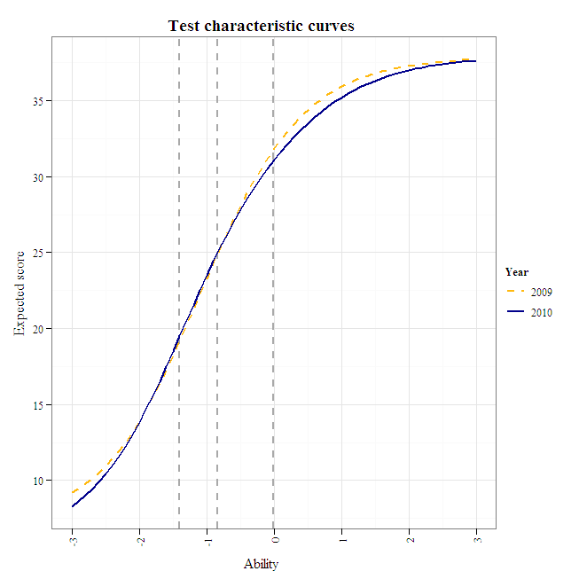
The test characteristic curves appear comparable up to the "exceeds proficiency standard" cut score, above which the test became more difficult compared to 2009.
########################################
#Plot overlapping conditional standard errors of measurement (from test information).
funk <- function(z) with(tif(z[, c("a", "b", "c")], x = thetas), data.frame(Ability = x, f))
data.plot <- ddply(data.pars, "year", funk)
data.plot$f <- 1/sqrt(data.plot$f)
g1 <- ggplot(data.plot, aes(x = Ability, y = f)) +
geom_vline(xintercept = cuts.grade3, linetype = 2, lwd = 1, color = "darkgrey") +
geom_line(aes(color = year, linetype = year), lwd = 1) +
scale_colour_manual(name = "Year", values = c("darkgoldenrod1", "darkblue")) +
scale_linetype_manual(name = "Year", values = 2:1) +
scale_y_continuous(name = "CSEM") +
opts(title = "Conditional standard errors of measurement")
g1
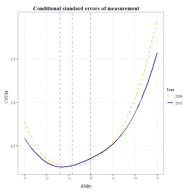
The conditional standard errors of measurement appear comparable, overall, except for the 2010 standard error at the exceeds-proficiency cut, which appears to slightly exceed the 0.25 rule of thumb.
########################################
#Plot overlapping CSEMs faceted by strand.
funk <- function(z) with(tif(z[, c("a", "b", "c")], x = thetas), data.frame(Ability = x, f))
data.plot <- ddply(data.pars, c("year", "strand"), funk)
data.plot$f <- 1/sqrt(data.plot$f)
g1 <- ggplot(data.plot, aes(x = Ability, y = f)) +
geom_vline(xintercept = cuts.grade3, linetype = 2, lwd = 1, color = "darkgrey") +
geom_line(aes(color = year, linetype = year), lwd = 1) +
scale_colour_manual(name = "Year", values = c("darkgoldenrod1", "darkblue")) +
scale_linetype_manual(name = "Year", values = 2:1) +
facet_wrap( ~ strand) +
scale_y_continuous(name = "CSEM") +
opts(title = "Conditional standard errors of measurement")
g1
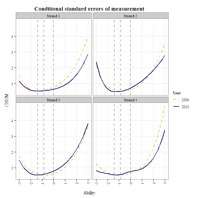
It looks like strand 3 could use a highly discriminating difficult item to bring its CSEM in line with the corresponding 2009 CSEM at the exceeds-proficiency cut.
########################################
#Plot item characteristic curves faceted by strand.
funk <- function(z) with(irf(z[, c("a", "b", "c")], x = thetas), data.frame(Ability = x, f))
data.plot <- ddply(data.pars, c("id", "year", "strand"), funk)
g1 <- ggplot(data.plot, aes(x = Ability, y = f)) +
geom_vline(xintercept = cuts.grade3, linetype = 2, lwd = 1, color = "darkgrey") +
geom_line(aes(group = id:year, color = year, linetype = year)) +
scale_colour_manual(name = "Year", values = c("darkgoldenrod1", "darkblue")) +
scale_linetype_manual(name = "Year", values = 2:1) +
facet_wrap( ~ strand) +
scale_y_continuous(name = "Probability", breaks = seq(0, 1, by = 0.25), limits = c(0, 1)) +
opts(title="Item characteristic curves")
g1
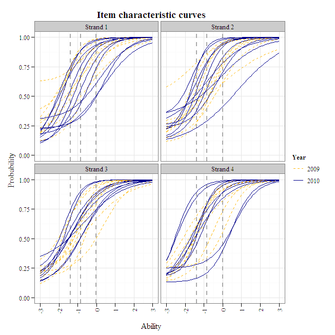
Compared to 2009, there are fewer items from strands 1 and 2 that students are able to guess easily (i.e., high c parameters/lower asymptotes). As noted above, strand 3 lacks an item that discriminates at the exceeds-proficiency cut. Replacing the poorly discriminating difficult item in strand 2 with a higher discriminating one would also reduce measurement error of high-ability students.