Creating accessible tables and graphs with R

I was recently given the task of improving the accessibility of a statistical report, with the goal of meeting level AA of the Web Content Accessibility Guidelines 2.0. The report contains about 600 pages of tables and graphs in a DOC file. The rule of thumb for tables is to ensure that a visually impaired person can use the tab key to navigate easily across cells in a row from the top left of the table to the bottom right. Additionally, tables and graphs should contain alternative titles and descriptions.

Last year, I produced the report with the Rlogo.jpg packages xtable and R2HTML. James Falkofske notes that hypertext markup language (HTML) files are inherently fluid, allowing readers with a wide range of abilities and assistive technologies to access the content. HTML tables with little or no nesting generally meet the navigation guidelines, even when opened with Word and saved as a word processor document. However, alternative titles and descriptions are not applied to tables and graphs automatically.

It would be very time consuming to retroactively add alternative text to 600 pages of tables and graphs in Word, so I decided to look for ways to modify the defaults in the xtable and R2HTML packages. The example below shows that it’s possible to add alternative text while writing tables and graphs to a HTML file. For tables, the goal is to add title and summary attributes to the <TABLE> tag. Those attributes will show up as alternative text when the HTML file is opened in Word. For graphs, the goal is to add title and “alt” attributes to the <IMG> tag. The graph’s “alt” attribute will carry over to the alternative description field when the HTML file is opened in Word, but the title won’t. However, adding title attributes will allow web browsers to display a float-over title for graphs as well as tables. Try it out by floating your cursor over the table and graph below.

########################################
#Load libraries.
library(xtable) #for tables
library(R2HTML) #for graphs
library(datasets) #for data
########################################
#Initiate a HTML file to export results.
#The file can be named with a DOC extension to facilitate opening it with Word.
name.file.htm <- "Accessible Tables and Graphs.doc"
HTML.title(
"Add alternative titles and descriptions to tables and graphs in a HTML-based DOC file",
file = name.file.htm, HR = 1, append = F)
########################################
#Accessible table example
#Assign alternative title and description to a single object.
html.table.attributes <- paste('border=1',
'title="Table of days of frost and years of life expectancy"',
'summary="Table of days of frost and years of life expectancy"')
#The xtable(caption) argument places the title in the first row of the table, making it
#more difficult to designate table headers to repeat across multiple pages in a document.
#Produce the table title with HTML.title() instead.
HTML.title("Days of frost and years of life expectancy", file = name.file.htm, HR = 3)
#Create table and write to file.
data.frost.exp <- as.data.frame(state.x77[, c("Frost", "Life Exp")])
names(data.frost.exp)[2] <- "Life"
table.xtable <- xtable(data.frost.exp, digits = c(NA, 0, 2))
print(table.xtable, type = "html", html.table.attributes = html.table.attributes,
file = name.file.htm, border = 1, append = T)
HTML("<br>", file = name.file.htm)
########################################
#Accessible graph example
#Modify HTMLInsertGraph() by adding Title and Alt arguments.
HTMLInsertGraph <- function (GraphFileName = "", Caption = "",
Title = "untitled graph", Alt = "a graph",
GraphBorder = 1, Align = "center",
WidthHTML = 500, HeightHTML = NULL,
file = get(".HTML.file"), append = TRUE, ...) {
cat("n", file = file, append = append, ...)
cat(paste("<p align=", Align, "><img src='", GraphFileName,
"' title='", Title, "' alt='", Alt, "' border=", GraphBorder,
if (!is.null(WidthHTML))
paste(" width=", WidthHTML, sep = "")
else "",
if (!is.null(HeightHTML))
paste(" height=", HeightHTML, sep = "")
else "", ">", sep = "", collapse = ""),
file = file, append = TRUE, sep = "")
if (Caption != "")
cat(paste("<br><i class=caption>", Caption, "</i>"),
file = file, append = TRUE, sep = "")
invisible(return(TRUE))
}
#Assign alternative title and description to objects.
Title <- "Graph of days of frost and years of life expectancy"
Alt <- "Graph of days of frost and years of life expectancy"
name.file.plot <- "Days of frost and years of life expectancy.png"
png(name.file.plot, width = 350, height = 350)
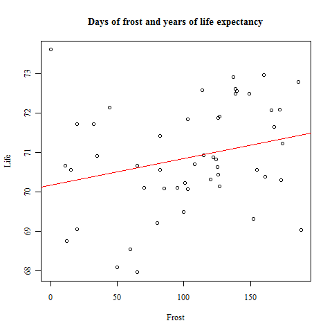
plot(data.frost.exp, main = "Days of frost and years of life expectancy", family = "serif")
abline(lm(Life ~ Frost, data.frost.exp), col = "red")
dev.off()
HTMLInsertGraph(GraphFileName = name.file.plot, file = name.file.htm, Align = "left",
WidthHTML = 350, HeightHTML = 350, append = T, Title = Title, Alt = Alt)
HTML("<br>", file = name.file.htm)

Days of frost and years of life expectancy

Frost Life
Alabama 20 69.05
Alaska 152 69.31
Arizona 15 70.55
Arkansas 65 70.66
California 20 71.71
Colorado 166 72.06
Connecticut 139 72.48
Delaware 103 70.06
Florida 11 70.66
Georgia 60 68.54
Hawaii 0 73.60
Idaho 126 71.87
Illinois 127 70.14
Indiana 122 70.88
Iowa 140 72.56
Kansas 114 72.58
Kentucky 95 70.10
Louisiana 12 68.76
Maine 161 70.39
Maryland 101 70.22
Massachusetts 103 71.83
Michigan 125 70.63
Minnesota 160 72.96
Mississippi 50 68.09
Missouri 108 70.69
Montana 155 70.56
Nebraska 139 72.60
Nevada 188 69.03
New Hampshire 174 71.23
New Jersey 115 70.93
New Mexico 120 70.32
New York 82 70.55
North Carolina 80 69.21
North Dakota 186 72.78
Ohio 124 70.82
Oklahoma 82 71.42
Oregon 44 72.13
Pennsylvania 126 70.43
Rhode Island 127 71.90
South Carolina 65 67.96
South Dakota 172 72.08
Tennessee 70 70.11
Texas 35 70.90
Utah 137 72.90
Vermont 168 71.64
Virginia 85 70.08
Washington 32 71.72
West Virginia 100 69.48
Wisconsin 149 72.48
Wyoming 173 70.29


Graph of days of frost and years of life expectancy

Posted in Praxes | Comments Off on Creating accessible tables and graphs with R

Best breweries in Minnesota: Value-added ratings

A good friend of mine told me to check out Beer Advocate online. Their rating system does a good job of balancing simplicity (A-F grades) with thoroughness (measures of central tendency and dispersion). I also appreciate the way it encourages raters and readers to consider multiple dimensions of a beer’s quality–its look, smell, taste, and feel–in addition to overall quality.

As a practitioner of multilevel and latent variable modeling, one aspect of Beer Advocate’s rating system has given me pause: a lack of adjustment for consistently high- or low-raters. What’s concerning about a simple average of ratings? Let’s imagine a plausible scenario: a motivated group of beer aficionados with high standards get their hands on a limited-release beer and publish their reviews on Beer Advocate. The beer could be world class, but if only tough raters have tried it, then the average rating will appear lower. Conversely, a large number of uncritical raters could review a mediocre beer, resulting in an excellent rating on average.

Is my concern warranted? If so, which beers and breweries are rated highest after adjusting for raters and other factors? To answer those questions, I wrote some Rlogo.jpg code to gather Beer Advocate ratings of beers produced by Minnesota breweries. The code relies heavily on the XML and stringr packages. After gathering the ratings, I decided to check my assumption of within-rater consistency. The intraclass correlation coefficient of r = 0.13 indicates a small degree of consistency within raters, but enough to justify my concern.

I specified a multilevel model to obtain value-added ratings of beers and breweries while adjusting for rater and beer characteristics. For simplicity, I decided to focus on the overall rating, although I would like to consider multiple dimensions of beer quality (look, smell, taste, and feel) in future analyses. The model specifies random effects for raters, cross-classified with beers nested in breweries. The fixed effects were the serving type experienced by the rater for a given beer (e.g., can), the beer’s alcohol by volume (ABV), and its style (e.g., porter).

.

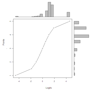
Note that I transformed the overall rating from a 1-5 scale to logits. I did so to avoid predictions below the floor of 1 point and above the ceiling of 5 points on the original scale (i.e., to enforce lower and upper asymptotes) and to spread the ratings out at the tails (e.g., make it “harder” to go from 4.5 to 5 than going from 3.5 to 4). The chart below shows the resulting ogival relationship between the original point system and the logits.

Plot showing transformation from points to logits
Points_to_Logits.png

I estimated the model parameters with the lme4 package. Given the large number of fixed effects (and the need for future blog content), I’ll describe the influence of serving type, ABV, and style at a later date. The value added by breweries after adjusting for rater and beer characteristics is shown in the table below. Value-added logits were transformed back to the original scale, with values in the table representing point deviations from the brewery average, but the logit and point ratings are virtually the same. August Schell Brewing Company recently won national accolades, but it came in second to a relative newcomer, Fulton Beer. Summit Brewing and Surly Brewing followed closely in the third and fourth spots. The results show some discrepancies between the value-added ratings and Beer Advocate’s grades, which are based on the simple average of all beer ratings. For example, Harriet Brewing received an A-, compared to Schell’s B grade, but Harriet’s value-added rating is below average.

Breweries sorted by value-added ratings
Brewery Value-added (logits) Value-added (points) Beer Advocate grade
(average beer rating)
Fulton Beer 0.85 0.80 A-
August Schell Brewing Co., Inc. 0.83 0.79 B
Summit Brewing Company 0.80 0.76 B+
Surly Brewing Company 0.71 0.68 A-
Minneapolis Town Hall Brewery 0.27 0.27 A-
Lake Superior Brewing Company 0.18 0.18 B
Fitger’s Brewhouse 0.10 0.10 B+
Olvalde Farm &amp Brewing Company 0.08 0.08 A-
Granite City Food &amp Brewery 0.04 0.04 B-
Flat Earth Brewing Company 0.03 0.03 B+
Brau Brothers Brewing Co., LLC 0.02 0.02 B
Pig’s Eye Brewing Company 0.00 0.00 D+
Harriet Brewing -0.09 -0.09 A-
Lift Bridge Brewery -0.11 -0.11 B+
Leech Lake Brewing Company -0.14 -0.14 B+
Barley John’s Brew Pub -0.26 -0.26 B+
McCann’s Food &amp Brew -0.27 -0.26 B+
St. Croix Brewing Company, LLC -0.69 -0.66 C
Cold Spring Brewing Co. -0.99 -0.91 D+
Great Waters Brewing -1.37 -1.19 B+


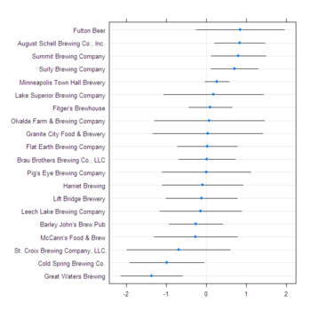
A different picture emerges when one considers that value-added ratings are point estimates within a range of certainty. The prediction-interval plot below shows that we can’t confidently conclude that Fulton Beer scored above average, let alone out performed Shell’s, Summit, or Surly. We can confidently say, though, that Shell’s, Summit, and Surly scored above average, and along with Minneapolis Town Hall Brewery, they significantly out-performed Cold Spring Brewing Co. and Great Waters Brewing.

Plot of breweries’ value-added ratings with 95% prediction intervals
Breweries_Value-Added.png

The results highlight some of the benefits of multilevel modeling and the limits of value-added ratings. By controlling for beer characteristics and separately estimating variance components for raters and beers nested in breweries, I have reduced the degree to which raters’ tastes and brewers’ preferences for certain types of beers are confounding brewery ratings. That is, the value-added ratings reflect the brewery’s overall quality with greater fidelity. Nevertheless, we should keep in mind that value-added ratings are based on error unexplained by theory/fixed effects, that they are point estimates within a range of certainty, and that one should interpret value-added ratings with caution because personal preferences still count. This analysis has motivated me to try beers by the breweries with high value-added ratings, but I know from experience that I like beers brewed by Brau Brothers, Lift Bridge, and Barley John’s, even though their value-added point estimates place them in the bottom half of Minnesota breweries.

Posted in Praxes | 1 Comment

Using irtoys, plyr, and ggplot2 for test development

My job as a Quantitative Analyst at the Minnesota Department of Education requires me to “provide evaluation, statistical, and psychometric support to the Division of Research and Assessment through the entire process of design, development, and reporting to the Minnesota assessment system.” That’s an accurate job description, but a little vague. What I really do is write a lot of Rlogo.jpg code to apply item response theory (IRT) and compare item and test characteristics across multiple years and/or forms to maintain high quality.

Rlogo.jpg is great for plotting item and test characteristics across multiple years and/or forms, but it requires using a few packages in concert (i.e., to my knowledge there is no single package designed for this purpose). The irtoys package provides many useful functions for test development under IRT; the plyr package allows one to apply irtoys’ functions to subsets of item parameters in a data set (e.g., by strand); and the ggplot2 package allows one to overlay and facet item and test curves.

In the following reproducible example, I graphically compare item and test characteristics of the 2009 and 2010 grade 3 Minnesota Comprehensive Assessments of reading ability. Note that for simplicity, I have excluded two polytomous items from 2009 and a few dichotomous items from 2010 from the published item parameter estimates. Also note that items have been assigned to strands arbitrarily in this example. Graphs such as these allow us to answer questions like, “Did the 2010 form yield as much information (i.e., measure with equal or less error) at the cut scores as the 2009 form?” The graphs also provide guidance for replacing undesirable items.

########################################
#Combine two years' worth of item parameter estimates from grade 3.
data.pars.2009 <- matrix(ncol = 3, byrow = T, c(0.57, -1.24, 0.17, 0.93, -0.74, 0.25,
1.45, -0.45, 0.19, 0.97, -0.5, 0.13, 0.95, -0.8, 0.62, 1.07, -0.38, 0.24, 0.87,
0.37, 0.22, 0.61, -1.45, 0.02, 0.84, -1.03, 0.19, 0.72, -0.23, 0.12, 0.93, -1.6,
0.25, 0.68, -2.02, 0.06, 1.1, -1.5, 0.36, 0.74, -1.6, 0.51, 1.01, -1.01, 0.21,
0.81, -1.52, 0.16, 0.93, -0.5, 0.11, 0.34, -0.75, 0.02, 0.92, -0.93, 0.19, 1.14,
0.21, 0.26, 0.54, -0.59, 0.1, 0.86, -0.52, 0.28, 1.04, -1.77, 0.05, 0.84, -1.68,
0.02, 1.46, -1.7, 0.17, 1.3, -1.16, 0.21, 0.51, -0.62, 0.1, 1.09, -1.04, 0.17,
0.66, -2.06, 0.09, 1.11, -0.61, 0.11, 1.34, -0.9, 0.26, 1.3, -1.24, 0.19, 1.37,
-1.72, 0.24, 1.09, -1.37, 0.16, 0.89, -0.94, 0.08, 1.24, -1.38, 0.14, 0.79, -1.32,
0.11, 1.09, -1.69, 0.13))
data.pars.2009 <- data.frame(2009, data.pars.2009)
names(data.pars.2009) <- c("year", "a", "b", "c")
data.pars.2009$strand <- factor(rep(1:4, length.out = 38), labels = paste("Strand", 1:4))
data.pars.2010 <- matrix(ncol = 3, byrow = T, c(1, -2.02, 0.05, 0.61, -0.88, 0.24,
0.74, -1.36, 0.08, 0.93, 0.63, 0.25, 0.94, 0.38, 0.23, 0.56, -0.14, 0.32, 0.7,
-0.73, 0.08, 1.1, -2.54, 0.02, 1.17, -0.36, 0.22, 0.46, 0.76, 0.09, 0.77, -1.53,
0.09, 1.5, -1.27, 0.18, 1.01, -1.41, 0.1, 1.63, -1.61, 0.21, 1.33, -1.63, 0.13,
1.11, -1.01, 0.19, 1.05, -1.17, 0.07, 0.88, -0.33, 0.23, 0.56, -0.65, 0.28, 1.03,
0.45, 0.13, 1.29, -1.73, 0.12, 0.96, -1.54, 0.15, 0.62, -1.33, 0.09, 0.67, -1.41,
0.06, 0.74, 0.16, 0.3, 1.33, -0.94, 0.26, 1.31, -1.71, 0.23, 1.14, -1.42, 0.16,
0.96, -0.87, 0.09, 1.22, -1.36, 0.14, 0.86, -1.19, 0.17, 0.94, -2.48, 0.02, 0.81,
-1.96, 0.02, 0.98, -0.86, 0.13, 0.8, -0.68, 0.11, 0.72, -1.67, 0.04, 0.63, 0.32,
0.16, 1.24, -1.64, 0.33))
data.pars.2010 <- data.frame(2010, data.pars.2010)
names(data.pars.2010) <- c("year", "a", "b", "c")
data.pars.2010$strand <- factor(rep(1:4, length.out = 38), labels = paste("Strand", 1:4))
data.pars <- rbind(data.pars.2009, data.pars.2010)
data.pars$year <- factor(data.pars$year)
data.pars$id <- factor(1:nrow(data.pars))
#Apply D scaling constant.
data.pars$a <- data.pars$a * 1.7
#Theta values for plotting
thetas <- seq(-3, 3, by = 0.1)
#Theta cut scores
cuts.grade3 <- c(-1.40, -0.84, -0.01)
########################################
#Plot overlapping test characteristic curves.
funk <- function(z) with(trf(z[, c("a", "b", "c")], x = thetas), data.frame(Ability = x, f))
data.plot <- ddply(data.pars, "year", funk)
g1 <- ggplot(data.plot, aes(x = Ability, y = f)) +
geom_vline(xintercept = cuts.grade3, linetype = 2, lwd = 1, color = "darkgrey") +
geom_line(aes(color = year, linetype = year), lwd = 1) +
scale_colour_manual(name = "Year", values = c("darkgoldenrod1", "darkblue")) +
scale_linetype_manual(name = "Year", values = 2:1) +
scale_y_continuous(name = "Expected score") +
opts(title = "Test characteristic curves")
g1

TCCs.png

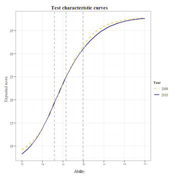
The test characteristic curves appear comparable up to the "exceeds proficiency standard" cut score, above which the test became more difficult compared to 2009.

########################################
#Plot overlapping conditional standard errors of measurement (from test information).
funk <- function(z) with(tif(z[, c("a", "b", "c")], x = thetas), data.frame(Ability = x, f))
data.plot <- ddply(data.pars, "year", funk)
data.plot$f <- 1/sqrt(data.plot$f)
g1 <- ggplot(data.plot, aes(x = Ability, y = f)) +
geom_vline(xintercept = cuts.grade3, linetype = 2, lwd = 1, color = "darkgrey") +
geom_line(aes(color = year, linetype = year), lwd = 1) +
scale_colour_manual(name = "Year", values = c("darkgoldenrod1", "darkblue")) +
scale_linetype_manual(name = "Year", values = 2:1) +
scale_y_continuous(name = "CSEM") +
opts(title = "Conditional standard errors of measurement")
g1

CSEMs.png

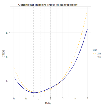
The conditional standard errors of measurement appear comparable, overall, except for the 2010 standard error at the exceeds-proficiency cut, which appears to slightly exceed the 0.25 rule of thumb.

########################################
#Plot overlapping CSEMs faceted by strand.
funk <- function(z) with(tif(z[, c("a", "b", "c")], x = thetas), data.frame(Ability = x, f))
data.plot <- ddply(data.pars, c("year", "strand"), funk)
data.plot$f <- 1/sqrt(data.plot$f)
g1 <- ggplot(data.plot, aes(x = Ability, y = f)) +
geom_vline(xintercept = cuts.grade3, linetype = 2, lwd = 1, color = "darkgrey") +
geom_line(aes(color = year, linetype = year), lwd = 1) +
scale_colour_manual(name = "Year", values = c("darkgoldenrod1", "darkblue")) +
scale_linetype_manual(name = "Year", values = 2:1) +
facet_wrap( ~ strand) +
scale_y_continuous(name = "CSEM") +
opts(title = "Conditional standard errors of measurement")
g1

CSEMs_Strand.png

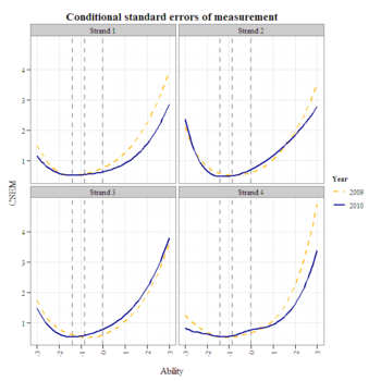
It looks like strand 3 could use a highly discriminating difficult item to bring its CSEM in line with the corresponding 2009 CSEM at the exceeds-proficiency cut.

########################################
#Plot item characteristic curves faceted by strand.
funk <- function(z) with(irf(z[, c("a", "b", "c")], x = thetas), data.frame(Ability = x, f))
data.plot <- ddply(data.pars, c("id", "year", "strand"), funk)
g1 <- ggplot(data.plot, aes(x = Ability, y = f)) +
geom_vline(xintercept = cuts.grade3, linetype = 2, lwd = 1, color = "darkgrey") +
geom_line(aes(group = id:year, color = year, linetype = year)) +
scale_colour_manual(name = "Year", values = c("darkgoldenrod1", "darkblue")) +
scale_linetype_manual(name = "Year", values = 2:1) +
facet_wrap( ~ strand) +
scale_y_continuous(name = "Probability", breaks = seq(0, 1, by = 0.25), limits = c(0, 1)) +
opts(title="Item characteristic curves")
g1

ICCs_Strand.png

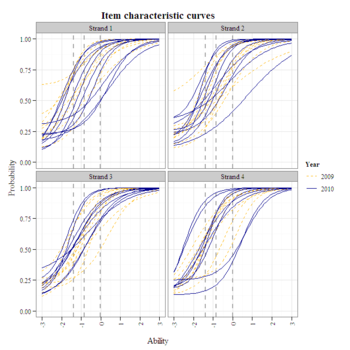
Compared to 2009, there are fewer items from strands 1 and 2 that students are able to guess easily (i.e., high c parameters/lower asymptotes). As noted above, strand 3 lacks an item that discriminates at the exceeds-proficiency cut. Replacing the poorly discriminating difficult item in strand 2 with a higher discriminating one would also reduce measurement error of high-ability students.

Posted in Praxes | Comments Off on Using irtoys, plyr, and ggplot2 for test development

My new nephews are way above average

Jacob_Outlier.jpg My new nephews, Jacob and Jadon, are way above average. And though they don’t even live in Lake Wobegon! See, it says so right on their onesies that I got from NausicaaDistribution.

Jadon_Outlier.jpg

Posted in Personal | Comments Off on My new nephews are way above average

Eastside Food Co-op goes solar

I love Eastside Food Co-op. They’re in my neighborhood and stock all my grocery needs. They show informative movies like “Troubled Waters: A Mississippi River Story,” which the University of Minnesota helped create but balked at showing. They hold community forums to discuss issues like pollution at Shoreham Yards. And they’ve welcomed Recovery Bike Shop into the building. A lot of great things are happening at Eastside Food Co-op.

To top it all off, Eastside Food Co-op has gone solar! Their solar panels began operating on December 8 and have generated over 160 killowat hours so far (see chart below). At at time when the Minnesota Legislature is considering nuclear power expansion, I am proud to belong to an organization that is investing in clean solar energy.

Eastside_Solar_Log.png

Posted in Personal | Comments Off on Eastside Food Co-op goes solar