I recently presented a paper on spatial regression discontinuity at the annual conference of the American Evaluation Association in Orlando. I wanted to graphically illustrate regression discontinuity and its spatial analogue, so I simulated some examples in ![]() . Plots such as these and William Trochim’s can be a good way to convey some of the key concepts of regression discontinuity design and analysis, such as curvilinear relationships between the assignment and outcome variable, local treatment effects, and the questionable validity of extrapolating program inferences beyond the cutoff.
. Plots such as these and William Trochim’s can be a good way to convey some of the key concepts of regression discontinuity design and analysis, such as curvilinear relationships between the assignment and outcome variable, local treatment effects, and the questionable validity of extrapolating program inferences beyond the cutoff.
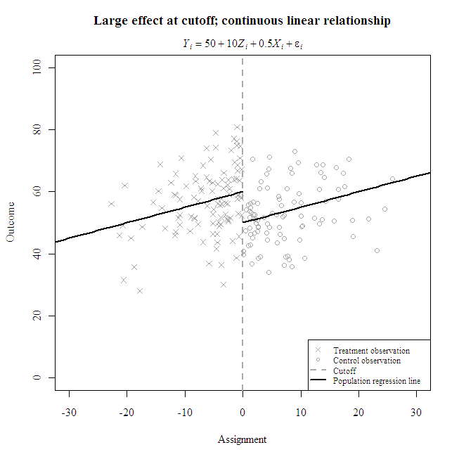
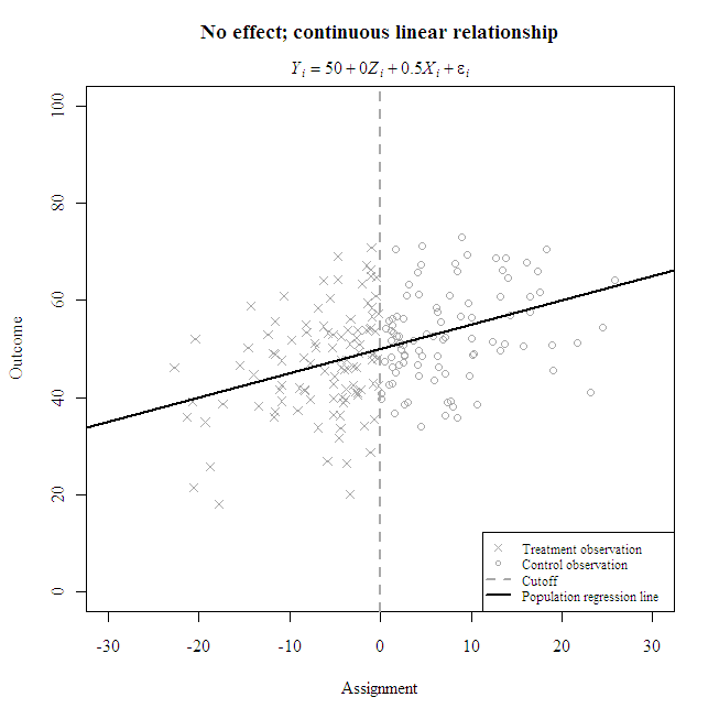
Local effect (left) and no effect (right) with continuous linear relationship between the assignment and outcome variable
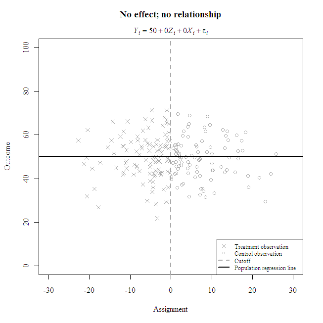
Average effect (left) and no effect (right) with no relationship between the assignment and outcome variable

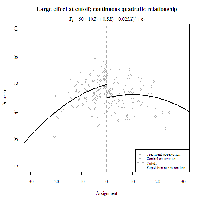
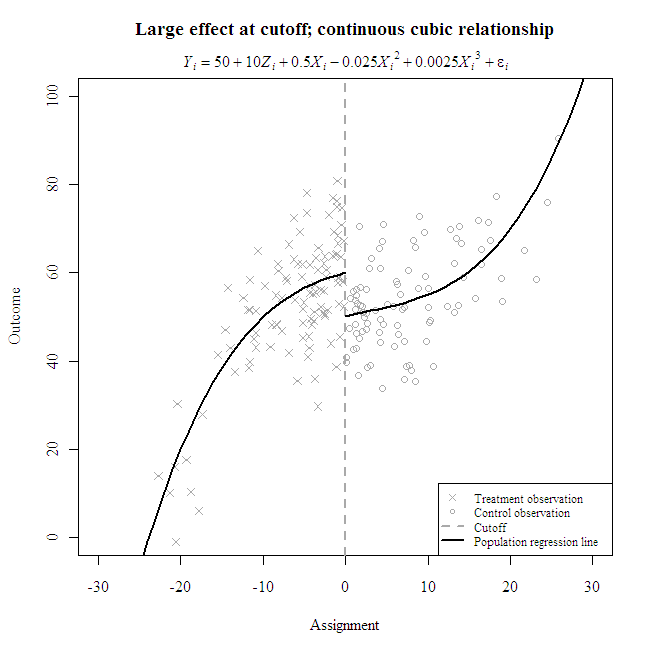
Local effects with curvilinear relationships between the assignment and outcome variable
Extrapolation: Local effect (left) and no local effect (right) with potentially larger effects beyond the cutoff due to discontinuous linear relationship between the assignment and outcome variable*
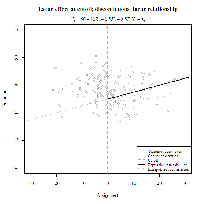
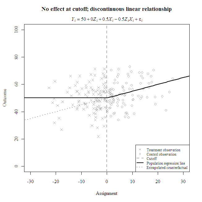
*Note: Extrapolations beyond the cutoff are rarely valid. Repetitious and abundant distal pretest observations may support extrapolating effect size estimates beyond the cutoff.
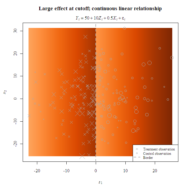
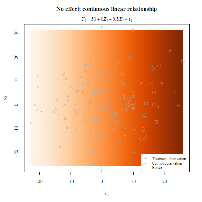
Spatial regression discontinuity: Local effect (left) and no effect (right) with continuous linear relationship between the assignment (distance from border) and outcome variable