Choosing a functional form for the relationship between the assignment and outcome variable from a regression discontinuity design is an important step in estimating the local average treatment effect. Plotting nonparametric smoothers can suggest a functional form, and nonparametric inference may be more appropriate when a curvilinear relationship defies classification. Some researchers exclusively prefer locally-weighted regression because they feel it objectively and conservatively excludes distal observations, although the choice of bandwidth can be subjective.
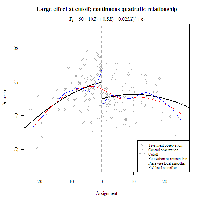
The following example shows a way to obtain and plot nonparametric estimates with ![]() . The approach yields an effect size estimate of about 2.1 standard deviations, which is over twice as large as the true effect (1 σ) and much worse than the parametric estimates (1.1 SD). Increasing the default span from 0.75 to 1 (not shown) improved the estimate slightly (1.3 SD), as did reducing it to 0.5 (1.6 SD). It would be interesting to conduct a simulation study to compare parametric and nonparametric effect size recovery over many random samples while systematically varying regression functions, bandwidths, and cutoff locations.
. The approach yields an effect size estimate of about 2.1 standard deviations, which is over twice as large as the true effect (1 σ) and much worse than the parametric estimates (1.1 SD). Increasing the default span from 0.75 to 1 (not shown) improved the estimate slightly (1.3 SD), as did reducing it to 0.5 (1.6 SD). It would be interesting to conduct a simulation study to compare parametric and nonparametric effect size recovery over many random samples while systematically varying regression functions, bandwidths, and cutoff locations.
#Simulate and plot the data as described in the first part of the previous entry.
#Use the full sample to fit a locally-weighted regression line.
lo <- loess(y ~ x, surface="direct")
x.lo <- min(x):max(x)
pred <- predict(lo, data.frame(x=x.lo))
lines(x.lo, pred, col="red")
#Use treatment observations to fit a locally-weighted regression line.
lo.tx <- loess(y ~ x, data.frame(y, x)[which(x<0),], surface="direct")
x.lo.tx <- 0:min(x)
pred.tx <- predict(lo.tx, data.frame(x=x.lo.tx))
lines(x.lo.tx, pred.tx, col="blue")
#Use control observations to fit a locally-weighted regression line.
lo.c <- loess(y ~ x, data.frame(y, x)[which(x>=0),], surface="direct")
x.lo.c <- 0:max(x)
pred.c <- predict(lo.c, data.frame(x=x.lo.c))
lines(x.lo.c, pred.c, col="blue")
#Add legend.
legend("bottomright", bg="white", cex=.75, pt.cex=.75, c("Treatment observation", "Control observation", "Cutoff", "Population regression line ", "Piecewise local smoother", "Full local smoother"), lty=c(NA, NA, 2, 1, 1, 1), lwd=c(NA, NA, 2, 2, 1, 1), col=c("darkgrey", "darkgrey", "darkgrey", "black", "blue", "red"), pch=c(4, 1, NA, NA, NA, NA))
#Nonparametric estimate [95% confidence interval] of local average treatement effect.
yhat.tx <- predict(lo.tx, 0, se=T)
yhat.c <- predict(lo.c, 0, se=T)
yhat.tx$fit - yhat.c$fit
c((yhat.tx$fit - qt(0.975, yhat.tx$df)*yhat.tx$se.fit) - (yhat.c$fit + qt(0.975, yhat.c$df)*yhat.c$se.fit), (yhat.tx$fit + qt(0.975, yhat.tx$df)*yhat.tx$se.fit) - (yhat.c$fit - qt(0.975, yhat.c$df)*yhat.c$se.fit))
Yields 21.28786 [7.453552, 35.122162].