Exploring dimensions of process quality measured by the Early Childhood Environment Rating Scale: Differential item functioning analysis

The Early Childhood Environment Rating Scale (Revised; ECERS-R) was designed to measure process quality in child care centers, but the data set that I have been analyzing contains ratings of center classrooms and family child care (FCC) homes. A sizable portion of the program’s budget was spent on training ECERS-R raters. Training them to reliably use both the ECERS-R and the Family Day Care Rating Scale (FDCRS) was cost prohibitive.

Was it unfair to rate FCC homes with the ECERS-R instrument? I conducted a differential item functioning (DIF) analysis to answer that question and remedy any apparent biases. Borrowing a quasi-experimental matching technique (not for the purpose of inferring causality), I employed propensity score weighting to match center classrooms with FCC homes of similar quality. For each item j, classroom/home i‘s propensity score (i.e., predicted probability of being an FCC home) was estimated using the following logistic regression model:

,

where FCC is a focal group dummy variable (1 if home; 0 if center) and Totalc stands for corrected total score (i.e., mean of item scores excluding item j). Classroom weights were calculated from the inverse of a site’s predicted probability of its actual type and normalized so the weights sum to the original sample size:

.

Such weights can induce overlapping distributions (i.e., balanced groups). In this case, the weights were were applied via weighted least squares (WLS) regression of item scores on corrected total scores and the focal group dummy, as well as an interaction term to consider the possibility of nonuniform/crossing DIF:

.

By minimizing , WLS gave classrooms/homes with weights greater than 1 more influence over parameter estimates and decreased the influence of those with weights less than 1.

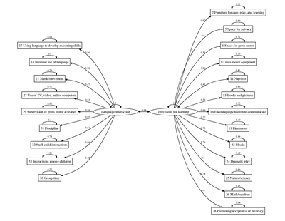
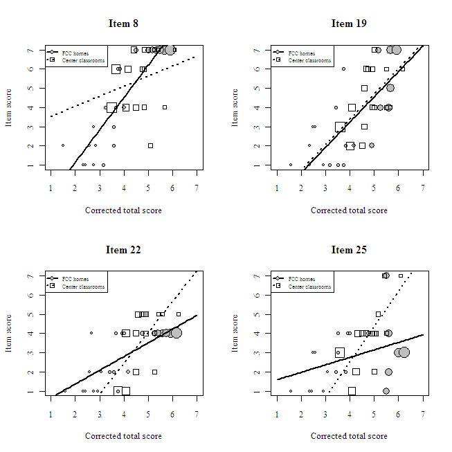
The results suggest that three provisions for learning items function differentially and in a non-uniform manner, as indicated by statistically significant interactions (see the table below). None of the language/interaction items exhibited DIF. The regression coefficients suggest that differentially functioning ECERS items did not consistently favor one type of care over the other. After dropping the three differentially functioning items from the provisions for learning scale and re-running the DIF analysis, none of the remaining items exhibited differential functioning.

Summary of WLS estimates: Differentially functioning ECERS items

Estimate Std. Error t value Pr(&gt |t|)
Item 8: Gross motor equipment
Intercept 3.014 2.044 1.475 0.149
Corrected total 0.523 0.445 1.175 0.248
FCC home -5.234 2.278 -2.297 0.028
Corrected*FCC 1.161 0.498 2.332 0.026
Item 22: Blocks
Intercept -3.990 1.919 -2.079 0.045
Corrected total 1.608 0.403 3.994 0.000
FCC home 3.929 2.076 1.892 0.067
Corrected*FCC -0.893 0.437 -2.045 0.049
Item 25: Nature/science
Intercept -4.802 2.566 -1.872 0.070
Corrected total 1.833 0.540 3.393 0.002
FCC home 5.996 2.771 2.164 0.038
Corrected*FCC -1.443 0.584 -2.471 0.019

Plot of weighted observations and fitted lines: Three crossing DIF items and one fair item (Item 19: Fine motor activities)
ECERS_DIF.png

Scores from the final provisions for learning scale exhibited good reliability of α = 0.87. Scores from the language/interaction scale also exhibited good reliability of α = 0.86. None of the items detracted problematically from overall reliability (i.e., the most that α increased after dropping any item was 0.01 in one instance).

I want to caution readers against generalizing the factor structure and DIF findings beyond this study because the sample is small in size (n = 38 classrooms/homes) and was drawn from a specific population (urban child care businesses subject to local market conditions and state-specific regulations). I largely avoided making statistical inferences in the preceding analyses by exploring the data and comparing relative fit, but in this case I used a significance level of 0.05 to infer DIF. The data do not provide a large amount of statistical power, so there could be more items that truly function differentially. For the final paper, I may apply a standardized effect size criterion. Standardized effect sizes are used to identify DIF with very large samples because the p-values would lead one to infer DIF for almost every item. De-emphasizing p-values in favor of effect sizes may be appropriate with small samples, too.

Posted in Praxes | Comments Off on Exploring dimensions of process quality measured by the Early Childhood Environment Rating Scale: Differential item functioning analysis

Exploring dimensions of process quality measured by the Early Childhood Environment Rating Scale: Confirmatory model comparison

I followed up the exploratory factor analysis (EFA) of the Early Childhood Environment Rating Scale (ECERS-R) with a confirmatory model comparison of the six-, two-, and one-factor solutions. The six-factor specification adhered to the original subscales in the ECERS-R instrument (after dropping highly skewed items); the two-factor specification simply restricted the minor loadings from the EFA to zero; and the one-factor specification restricted items to zero if they loaded less than |0.3| in the one-factor EFA solution.

The six-factor model did not converge, and the two-factor model exhibited better fit than the one-factor model. These results support earlier findings by Sakai and colleagues (2003) and Cassidy and colleagues (2005) that the ECERS-R measures two latent factors: provisions for learning and language/interaction experienced by children.

The goal of this analysis was to find a factorially simple solution. Higher order or hierarchical models of greater complexity would be worth considering in light of evolving theories and needs surrounding measures of child care quality and given that:

  • several ECERS-R items cross-loaded in the EFAs and were subsequently excluded
  • the overall fit of the two-factor model was poor
  • the estimated correlation between the latent factors was somewhat large (0.68).

Comparison of one- and two-factor models

CFA fit measure One factor Two factors
Model χ2 750, df = 377, p < 0.01 306, df = 208, p < 0.01
χ2 (null model) 1139, df = 406 653, df = 231
Goodness-of-fit index 0.509 0.645
Adjusted goodness-of-fit index 0.433 0.569
RMSEA index 0.164 0.113
Bentler-Bonnett NFI 0.341 0.532
Tucker-Lewis NNFI 0.452 0.742
Bentler CFI 0.491 0.768
SRMR 0.115 0.107
BIC -621 -451

Measurement model (click image)
ECERS_Path_Diagram.png

Posted in Praxes | Comments Off on Exploring dimensions of process quality measured by the Early Childhood Environment Rating Scale: Confirmatory model comparison

Exploring dimensions of process quality measured by the Early Childhood Environment Rating Scale

The Early Childhood Environment Rating Scale, revised edition (ECERS-R; Harms, Clifford, & Cryer, 1998), is an instrument used widely to observe and rate levels of process quality in child care centers. The authors have divided the instrument into six subscales to help ensure broad and flexible coverage of various aspects of child care quality. (The ECERS-R actually contains seven subscales, but the last one pertains to parents and staff instead of process quality experienced by children.) Psychometric analyses suggest the ECERS-R actually measures two latent dimensions of quality at most. Perlman, Zellman, and Le (2004) concluded that process quality, as measured by the ECERS-R, is unidimensional. Sakai and colleagues (2003) and Cassidy and colleagues (2005) concluded that the ECERS-R measures two latent dimensions, although their factor loadings and interpretations differ across the two studies.

I am writing a paper to present at the upcoming American Educational Research Association (AERA) conference in Denver. The paper will report results from a structural equation mediation model of the influence of on-site child care professional development on school readiness through child care quality. Given the lack of agreement among the earlier psychometric analyses of the ECERS-R, I conducted an exploratory factor analysis to see if I could replicate findings from one of the earlier studies. As shown in the table below, my preliminary results and interpretations do not align perfectly with either of the two-factor solutions from the earlier studies, but the similarities helped me decide which items to drop and which of my interpretations to keep. I plan to use a confirmatory factor analysis to formally compare model fit between the one- and two-factor solution before estimating the mediation model. I hope the summary below will help others who are wrestling with the possibility of multiple dimensions of child care quality as measured by the ECERS-R.

Summary of ECERS-R two-factor solutions from three studies

Item number Item Subscale Sakai and colleagues (2003) Cassidy and colleagues (2005) Moore (2010) Decision
1 Indoor space Space and furnishings Provisions for learning     Drop
2 Furniture for care, play, and learning Space and furnishings Teaching and interactions   Provisions for learning Discrepancy
3 Furnishings for relaxation Space and furnishings Teaching and interactions Materials/activities   Discrepancy
4 Room arrangement Space and furnishings Provisions for learning     Drop
5 Space for privacy Space and furnishings   Materials/activities Provisions for learning Keep
6 Space for gross motor Space and furnishings     Provisions for learning Discrepancy
7 Child-related display Space and furnishings Teaching and interactions     Drop
8 Gross motor equipment Space and furnishings Provisions for learning   Provisions for learning Keep
9 Greeting/departing Personal care routines Teaching and interactions     Drop
10 Meals/ snacks Personal care routines Provisions for learning     Drop
11 Nap/rest Personal care routines     Provisions for learning Discrepancy
12 Toileting/diapering Personal care routines Provisions for learning     Drop
13 Health practices Personal care routines Provisions for learning     Drop
14 Safety practices Personal care routines Provisions for learning     Drop
15 Books and pictures Language-reasoning Provisions for learning Materials/activities Provisions for learning Keep
16 Encouraging children to communicate Language-reasoning     Provisions for learning Discrepancy
17 Using language to develop reasoning skills Language-reasoning Teaching and interactions Language/interaction Language/interaction Keep
18 Informal use of language Language-reasoning Teaching and interactions Language/interaction Language/interaction Keep
19 Fine motor Activities Teaching and interactions Materials/activities Provisions for learning Keep
20 Art Activities   Materials/activities   Drop
21 Music/movement Activities Teaching and interactions   Language/interaction Keep
22 Blocks Activities Provisions for learning Materials/activities Provisions for learning Keep
23 Sand/water Activities Provisions for learning     Drop
24 Dramatic play Activities Provisions for learning Materials/activities Provisions for learning Keep
25 Nature/science Activities   Materials/activities Provisions for learning Keep
26 Math/numbers Activities Teaching and interactions Materials/activities Provisions for learning Keep
27 Use of TV, video, and/or computers Activities     Language/interaction Discrepancy
28 Promoting acceptance of diversity Activities Provisions for learning   Provisions for learning Keep
29 Supervision of gross motor activities Interaction     Language/interaction Discrepancy
30 General supervision of children Interaction Provisions for learning Language/interaction   Discrepancy
31 Discipline Interaction   Language/interaction Language/interaction Keep
32 Staff-child interactions Interaction Provisions for learning Language/interaction Language/interaction Keep
33 Interactions among children Interaction Teaching and interactions Language/interaction Language/interaction Keep
34 Schedule Program structure Provisions for learning     Drop
35 Free play Program structure Teaching and interactions     Drop
36 Group time Program structure Provisions for learning Language/interaction Language/interaction Keep

Note: Empty cells indicate loadings less than |0.3|, cross-loadings greater than |0.3|, or items skewed greater than |2|. Item 37, which asks about provisions for children with disabilities was excluded due to high missingness.

Posted in Praxes | Comments Off on Exploring dimensions of process quality measured by the Early Childhood Environment Rating Scale

Kettle River ski trip

Here are some pictures from a ski trip that Amy and I took to Banning State Park. It was our first trip to Banning. We stopped there on our way to the Wilco show in Duluth. We met several friendly people along the trails who agreed that Banning is underrated. The trails were well-maintained and covered a diverse mix of terrain and cultural artifacts along the Kettle River, including the historic Sandstone Quarry. The Kettle is one of the few whitewater rivers in Minnesota. I hope to paddle it someday, especially after seeing it up close. I’m an awful skier, but cross country skiing is a great way to enjoy the frozen lakes and rivers until they thaw. (If you can’t canoe it, you might as well ski it!) Amy, on the other hand, is a powerhouse skier who competed for her high school team.

IMG_0840.jpg IMG_0841.jpg
IMG_0813.jpg IMG_0798.jpg
IMG_0842.jpg IMG_0845.jpg

Posted in Personal | Comments Off on Kettle River ski trip

Multilevel Rasch: Estimation with R

My last post described how test development designs could be thought of as multistage sampling designs and how multilevel Rasch could be used to estimate parameters under that assumption. I decided to use Rlogo.jpg to compare estimates from the usual Rasch model, the generalized linear model (GLM) with a logit link, and generalized linear mixed-effects regression (GLMER), treating items as fixed then random effects. The GLMER model with item fixed effects exhibited the best fit of the Law School Admission Test (LSAT) data provided with the ltm package. Moreover, intraclass correlation has reduced the effective sample size relative to simple random sampling, lending further support to the multilevel Rasch approach.

#Load libraries.
library(ltm)
library(lme4)
library(xtable)

#Prepare data for GLM.
LSAT.long <- reshape(LSAT, times=1:5, timevar="Item", varying=list(1:5), direction="long")
names(LSAT.long) <- c("Item", "Score", "ID")
LSAT.long$Item <- as.factor(LSAT.long$Item)
LSAT.long$ID <- as.factor(LSAT.long$ID) #Compute Rasch, GLM, and GLMER estimates and compare fit.
out.rasch <- rasch(LSAT, constraint=cbind(ncol(LSAT)+1, 1))
print(xtable(summary(out.rasch)$coefficients, digits=3), type="html")

value std.err z.vals
Dffclt.Item1 -2.872 0.129 -22.307
Dffclt.Item2 -1.063 0.082 -12.946
Dffclt.Item3 -0.258 0.077 -3.363
Dffclt.Item4 -1.388 0.086 -16.048
Dffclt.Item5 -2.219 0.105 -21.166
Dscrmn 1.000


out.glm <- glm(Score ~ Item, LSAT.long, family="binomial")
print(xtable(summary(out.glm)$coefficients, digits=3), type="html")

Estimate Std. Error z value Pr(&gt |z|)
(Intercept) 2.498 0.119 20.933 0.000
Item2 -1.607 0.138 -11.635 0.000
Item3 -2.285 0.135 -16.899 0.000
Item4 -1.329 0.141 -9.450 0.000
Item5 -0.597 0.152 -3.930 0.000


out.glmer <- glmer(Score ~ Item + (1|ID), LSAT.long, family="binomial")
print(xtable(summary(out.glmer)@coefs, digits=3, caption="Fixed effects"), type="html", caption.placement="top")
print(xtable(summary(out.glmer)@REmat, digits=3, caption="Random effects"), type="html", caption.placement="top", include.rownames=F)

Fixed effects
Estimate Std. Error z value Pr(&gt |z|)
(Intercept) 2.705 0.129 21.029 0.000
Item2 -1.711 0.145 -11.774 0.000
Item3 -2.467 0.142 -17.353 0.000
Item4 -1.406 0.148 -9.498 0.000
Item5 -0.623 0.160 -3.880 0.000

Random effects
Groups Name Variance Std.Dev.
ID (Intercept) 0.502 0.70852


out.glmer.re <- glmer(Score ~ (1|Item) + (1|ID), LSAT.long, family="binomial")
print(xtable(summary(out.glmer.re)@coefs, digits=3, caption="Fixed effects"), type="html", caption.placement="top")
print(xtable(summary(out.glmer.re)@REmat[,-6], digits=3, caption="Random effects"), type="html", caption.placement="top", include.rownames=F)

Fixed effects
Estimate Std. Error z value Pr(&gt |z|)
(Intercept) 1.448 0.379 3.818 0.000


Random effects
Groups Name Variance Std.Dev.
ID (Intercept) 0.45193 0.67226
Item (Intercept) 0.70968 0.84243


print(xtable(AICs.Rasch.GLM <- data.frame(Rasch=summary(out.rasch)$AIC, GLM=summary(out.glm)$aic, GLMER.fe=summary(out.glmer)@AICtab$AIC, GLMER.re=summary(out.glmer.re)@AICtab$AIC, row.names="AIC"), caption="Akaike's information criteria (AICs)"), type="html", caption.placement="top")

Akaike’s information criteria (AICs)
Rasch GLM GLMER.fe GLMER.re
AIC 4956.11 4996.87 4950.80 4977.25


#Easiness estimates.
easiness <- data.frame(Rasch=out.rasch$coefficients[,1],
GLM=c(out.glm$coefficients[1], out.glm$coefficients[1]+out.glm$coefficients[-1]),
GLMER.fe=c(fixef(out.glmer)[1], fixef(out.glmer)[1]+fixef(out.glmer)[-1]),
GLMER.re=fixef(out.glmer.re)+unlist(ranef(out.glmer.re)$Item))
print(xtable(easiness, digits=3), type="html")

Rasch GLM GLMER.fe GLMER.re
Item 1 2.872 2.498 2.705 2.527
Item 2 1.063 0.891 0.994 0.917
Item 3 0.258 0.213 0.237 0.224
Item 4 1.388 1.169 1.299 1.201
Item 5 2.219 1.901 2.082 1.938


#Estimated probabilities of a correct response.
pr.correct <- sapply(easiness, plogis)
row.names(pr.correct) <- row.names(easiness)
print(xtable(pr.correct, digits=3), type="html")

Rasch GLM GLMER.fe GLMER.re
Item 1 0.946 0.924 0.937 0.926
Item 2 0.743 0.709 0.730 0.714
Item 3 0.564 0.553 0.559 0.556
Item 4 0.800 0.763 0.786 0.769
Item 5 0.902 0.870 0.889 0.874


#Difficulty estimates.
difficulties <- easiness*-1
print(xtable(difficulties, digits=3), type="html")

Rasch GLM GLMER.fe GLMER.re
Item 1 -2.872 -2.498 -2.705 -2.527
Item 2 -1.063 -0.891 -0.994 -0.917
Item 3 -0.258 -0.213 -0.237 -0.224
Item 4 -1.388 -1.169 -1.299 -1.201
Item 5 -2.219 -1.901 -2.082 -1.938


#Calculate design effects and effective samples sizes from intraclass correlation coefficients and sampling unit sizes.
multistage.consequences <- function(ICC, N) {
M <- nrow(LSAT.long)
n <- M/N #number of responses per item
deff <- 1+(n-1)*ICC
M.effective <- trunc(M/deff)
return(data.frame(ICC, M, N, n, deff, M.effective))
}
model.ICC.Item <- glmer(Score ~ 1 + (1|Item), family=binomial, data=LSAT.long)
ICC.Item <- as.numeric(VarCorr(model.ICC.Item)$Item)/(as.numeric(VarCorr(model.ICC.Item)$Item)+pi^2/3)
multistage.Item <- multistage.consequences(ICC.Item, 5)
model.ICC.ID <- glmer(Score ~ 1 + (1|ID), family=binomial, data=LSAT.long)
ICC.ID <- as.numeric(VarCorr(model.ICC.ID)$ID)/(as.numeric(VarCorr(model.ICC.ID)$ID)+pi^2/3)
multistage.ID <- multistage.consequences(ICC.ID, 1000)
multistage <- data.frame(cbind(t(multistage.Item), t(multistage.ID)))
names(multistage) <- c("Item", "ID")
print(xtable(multistage, digits=3), type="html")

Item ID
ICC 0.159 0.070
M 5000.000 5000.000
N 5.000 1000.000
n 1000.000 5.000
deff 160.295 1.281
M.effective 31.000 3903.000


#Plot test characteristic curves
plot.tcc <- function(difficulties, add, col, lty) {
thetas <- seq(-3.8,3.8,length=100)
temp <- matrix(nrow=length(difficulties), ncol=length(thetas))
for(i in 1:length(thetas)) {for(theta in thetas) temp[,which(thetas==theta)] <- plogis(theta-difficulties)}
if(missing(add)) {plot(thetas, colSums(temp), ylim=c(0,5), col=NULL, ylab=expression(tau), xlab=expression(theta), main="Test characteristic curves")}
lines(thetas, colSums(temp), col=col, lty=lty)
}
plot.tcc(difficulties=difficulties[,1], col="black", lty=1)
plot.tcc(difficulties=difficulties[,2], add=T, col="blue", lty=2)
plot.tcc(difficulties=difficulties[,3], add=T, col="red", lty=3)
plot.tcc(difficulties=difficulties[,4], add=T, col="green", lty=4)
legend("bottomright", c("Rasch", "GLM", "GLMER, fixed items", "GLMER, random items "), col=c("black", "blue", "red", "green"), lty=1:4)

Multilvel_Rasch_Test_Characteristic_Curves.png

Posted in Praxes | 2 Comments