Anniversary trip: Lake Pepin and Zumbro River

00000026.JPG

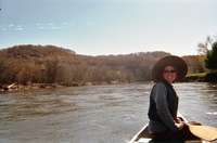
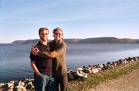
Amy and I celebrated our eighth anniversary with a trip to southeastern Minnesota. The forecast called for warm and sunny weather, so we decided to camp and canoe. We wanted to camp at Frontenac State Park to get some more mileage out of our state park pass, but the fall colors and warm weather helped fill up Frontenac’s campground. One of the park rangers recommended Hok-Si-La Campground in Lake City. It was a fantastic campground with well-kept facilities and campsites right on Lake Pepin’s shore. During breakfast in our campsite we saw several species of birds, including a bald eagle and a downy woodpecker.

00000014.JPG

For our canoe trip, we chose a section of the Zumbro River from Theillman to river mile 13 near Dumfries. We chose that route because much of it is protected as part of the Richard J. Dorer Memorial Hardwood State Forest. Riverland Outfitters shuttled us to the put-in. A month before our trip, flooding devastated towns along the Zumbro River. Although the waters had receded well below flood stage, the river was still running at a brisk pace. It took us about six hours to cover 13 river miles on the Buffalo and Nemadji Rivers, but it only took about three hours on the Zumbro. We enjoyed the views of the hillsides and farms, the sand bars, and dodging all the submerged trees in the river. According to Paddling Minnesota, the Zumbro derives its name from the French pronunciation of “embarrassment” caused by the river’s obstacles.

00000006.JPG

After getting off the water, we walked around downtown Wabasha before heading across the river to Pepin, Wisconsin, for an anniversary dinner at the Harbor View Cafe. The cafe was hopping. It took about two hours to get a table. We didn’t mind because it gave us a chance to walk around the harbor and listen to some live jazz and folk music outside the pub next door. Harbor View Cafe was overpriced for the quality of the food and service, but the overall experience of visiting and dining in Pepin made it worthwhile. The great company and occasion made for a memorable experience.

Posted in Personal | Comments Off on Anniversary trip: Lake Pepin and Zumbro River

Urban canoeing: Lake Phalen to Gervais Lake

Phalen_Gervais (2).jpg Phalen_Gervais (6).jpg

Here are some pictures from a nice little canoeing trip we took with our friend, Jim. He owns a beautiful wood canvas canoe. The three of us became friends at YMCA Camp Widjiwagan in Ely, where wood canvas canoes are used as part of the curriculum to teach young people about teamwork and environmental stewardship. In addition to being easy on the eye, wood canvas canoes are very quiet on the water–much quieter than Scrappy, our aluminum canoe.

Phalen_Gervais (0).jpg

It was nice to spend some time in the Payne-Phalen neighborhood of Saint Paul. We hardly make it over there. We put in at Lake Phalen, padded through Phalen Park, portaged around a bridge repair project to Round Lake, paddled along a scenic creek leading to Keller Lake, and then paddled under Highway 36 into Gervais Lake. It was getting dark, so we didn’t spend much time on Gervais Lake before heading back to the put-in. People gush about the Minneapolis chain of lakes, but the Phalen-Gervais chain of lakes is quite nice, too. Some highlights: water fowl, families enjoying the park, ice cream truck, many bridges, kayakers practicing rolling, fall leaves, quiet canoe, spending time with a good friend.

Posted in Personal | Comments Off on Urban canoeing: Lake Phalen to Gervais Lake

Plotting survey responses representing three or more dimensions

Bob Williams recently posted a question to EVALTALK about open source software for plotting survey responses in three dimensions:

I’m wondering how to display Likert scale data in three dimensions (ie the Likert scores for each subject on 3 scale dimensions). My graphic software is not that sophisticated and I haven’t been able to find an open source equivalent…. that can plot something along three dimensions (X,Y,Z) like this:

          X, Y, Z
Subject A 2, 5, 8
Subject B 3, 5, 9
Subject C 3, 7, 3

Another evaluator, Bill Harris, recommended Rlogo.jpg and ggplot2 in particular.

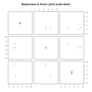
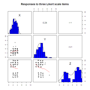
Bob’s question and the mention of Rlogo.jpg inspired me to write up a brief demonstration of plotting multi-dimensional data. As I have mentioned in the past (see here, here, and here), plotting or mapping three or more dimensions can be difficult and potentially misleading because plots and maps are inherently two-dimensional. I would say that plotting three survey response dimensions actually requires plotting four dimensions: X, Y, Z, and the frequency of each X, Y, and Z combination. That’s because evaluators commonly have large data sets with repeated response patterns. I simulated a larger data set from Bob’s example in order to illustrate plotting four dimensions.

#Open a recording window (if using Windows).
windows(record=T)
#Manually read in the data.
data.3D <- data.frame(Subject = c("A", "B", "C"),
X = c(2, 3, 3),
Y = c(5, 5, 7),
Z = c(8, 9, 3))
data.3D
#Larger data sets will contain frequently repeated combinations of responses.
#Simulate a larger data set with repeated responses combinations.
data.4D <- data.3D
for(i in 1:200) {
temp <- data.frame(Subject=factor(paste(as.character(data.3D[, 1]), i, sep=".")),
X=round(jitter(data.3D[, 2], 7), 0),
Y=round(jitter(data.3D[, 2], 7), 0),
Z=round(jitter(data.3D[, 4], 7), 0))
data.4D <- rbind(data.4D, temp)
}
library(plyr)
data.4D <- ddply(data.4D, c("X", "Y", "Z"), "nrow")
names(data.4D)[which(names(data.4D)=="nrow")] <- "Frequency"
data.4D <- data.4D[order(data.4D$Frequency, decreasing=T), ]
#Scatterplot matrices
pairs(data.3D[2:4], xlim=c(0, 10), ylim=c(0, 10),
main="Responses to three Likert scale items")
library(psych)
pairs.panels(sapply(data.4D[1:3], jitter), xlim=c(0, 10), ylim=c(0, 10), ellipses=F,
hist.col="blue", pch=1, scale=T, main="Responses to three Likert scale items")
Scatterplot_Matrix1_EVALTALK.png Scatterplot_Matrix2_EVALTALK.png

#Load ggplot2 library; set theme without gray background.
library(ggplot2)
theme_set(theme_bw())
#Create a scatterplot with size and color varying by the third dimension.
plot1 <- ggplot(data=data.3D, aes(x=X, y=Y, color=Z, size=Z)) +
geom_point() +
xlim(0, 10) +
ylim(0, 10) +
scale_colour_gradient(breaks=0:10, limits=c(0, 10), low="lightblue", high="darkblue") +
scale_size_continuous(breaks=0:10, limits=c(0, 10)) +
opts(title="Responses to three Likert scale items")
plot1
#Create a jittered scatterplot with color varying by the third dimension
#and size by response combination frequency.
plot2 <- ggplot(data=data.4D, aes(x=X, y=Y, color=Z, size=Frequency)) +
geom_jitter() +
xlim(0, 10) +
ylim(0, 10) +
scale_colour_gradient(breaks=0:10, limits=c(0, 10), low="lightblue", high="darkblue") +
scale_size_continuous() +
opts(title="Responses to three Likert scale items")
plot2
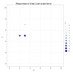
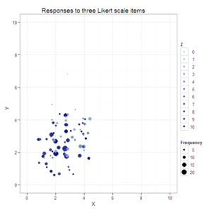
ggplot1_EVALTALK.png ggplot2_EVALTALK.png

#Reshape data from wide to longer.
data.3D.longer <- melt(data.3D, id.vars=c("Subject", "Y"), variable_name="Item")
names(data.3D.longer)[which(names(data.3D.longer)=="value")] <- "Response"
data.3D.longer
#Create a scatterplot with faceted second and third dimensions.
plot3 <- ggplot(data=data.3D.longer, aes(x=Response, y=Y)) +
geom_point(color="blue") +
xlim(0, 10) +
ylim(0, 10) +
facet_grid(. ~ Item) +
opts(title="Responses to three Likert scale items")
plot3
#Reshape simulated data from wide to longer.
data.4D.longer <- melt(data.4D, id.vars=c("Y", "Frequency"), variable_name="Item")
names(data.4D.longer)[which(names(data.4D.longer)=="value")] <- "Response"
head(data.4D.longer)
#Create a scatterplot with faceted second and third dimensions
#and size varying by response combination frequency.
plot4 <- ggplot(data=data.4D.longer, aes(x=Response, y=Y, size=Frequency)) +
geom_jitter(color="blue") +
xlim(0, 10) +
ylim(0, 10) +
facet_grid(. ~ Item) +
opts(title="Responses to three Likert scale items")
plot4
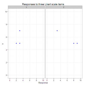
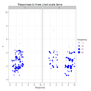
ggplot3_EVALTALK.png ggplot4_EVALTALK.png

Posted in Praxes | Comments Off on Plotting survey responses representing three or more dimensions

KFAI rocks

I want to give a shout-out to KFAI, Fresh Air Community Radio. I listen to KFAI just about every day. And every day I am impressed by the station’s diverse programming and skilled volunteer DJs. I urge everyone to tune into 90.3 in Minneapolis, 106.7 in Saint Paul, or on the Web at http://www.kfai.org. Then support them with a contribution. Here’s a list of my favorite shows to get you started:

  1. African Rhythms
  2. Sugar Shop
  3. Sangam
  4. Caribbean Jam
  5. Mostly Jazz
  6. Blueslady’s Time Machine
  7. Louisiana Rhythms
Posted in Personal | Comments Off on KFAI rocks

Linear mixed-effects regression p-values in R: A likelihood ratio test function

Following Douglas Bates’ advice for those required to produce p-values for fixed-effects terms in a mixed-effects model, I wrote a function to perform a likelihood ratio test for each term in an lmer() object. Bates has championed the notion that calculating the p-values for fixed effects is not trivial. That’s because with unbalanced, multilevel data, the denominator degrees of freedom used to penalize certainty are unknown (i.e., we’re uncertain about how uncertain we should be). As the author of lme4, the foremost mixed-effects modeling package in Rlogo.jpg, he has practiced what he preaches by declining to approximate denominator degrees of freedom as SAS does. Bates contends that alternative inferential approaches make p-values unnecessary. I agree with that position, focusing instead on information criteria and effect sizes. However, as a program evaluator, I recognize that some stakeholders find p-values useful for understanding findings.

A likelihood ratio test can be used to test if the sample size is large. According to Fitzmaurice, Laird, and Ware, twice the difference between the maximized log-likelihoods of two nested models, , represents the degree to which the reduced model is inadequate. When the sample size is large, with degrees of freedom equal to the difference in parameters between the full and reduced models, . The p-value is will be too liberal (i.e., the type I error rate will exceed the nominal p-value). More conservatively, we might say that with numerator and denominator degrees of freedom. According to Snijders and Bosker, the effective sample size lies somewhere between total micro-observations (i.e., at level one) and clusters randomly sampled in earlier stages (i.e., at higher levels). Formally, the effective sample size is , where observations are nested within each cluster and intraclass correlation is . Even if is large, (and statistical power) could be quite small if is small and is large: . Unbalanced designs, modeling three or more levels, and cross-level interactions add to our uncertainty about the denominator degrees of freedom.

The function I wrote chews up the lmer() model call and concatenates the frame and model matrix slots, after which it iteratively fits (via maximum likelihood instead of restricted ML) models reduced by each fixed effect and compares them to the full model, yielding a vector of p-values based on . As the example shows, the function can handle shortcut formulas whereby lower order terms are implied by an interaction term. The function doesn’t currently handle weights, glmer() objects, or on-the-fly transformations of the dependent variable [e.g., log(dep.var) ~ ...]. The accuracy of resulting p-values depends on large sample properties, as discussed above, so I don’t recommend using the function with small samples. I’m working on another function that will calculate p-values based on the effective sample size estimated from intraclass correlation. I will post that function in a future entry. I’m sure the following function could be improved, but I wanted to go ahead share it with other applied researchers whose audience likes p-values. Please let me know if you see ways to make it better.

p.values.lmer <- function(x) {
summary.model <- summary(x)
data.lmer <- data.frame(model.matrix(x))
names(data.lmer) <- names(fixef(x))
names(data.lmer) <- gsub(pattern=":", x=names(data.lmer), replacement=".", fixed=T)
names(data.lmer) <- ifelse(names(data.lmer)=="(Intercept)", "Intercept", names(data.lmer))
string.call <- strsplit(x=as.character(x@call), split=" + (", fixed=T)
var.dep <- unlist(strsplit(x=unlist(string.call)[2], " ~ ", fixed=T))[1]
vars.fixef <- names(data.lmer)
formula.ranef <- paste("+ (", string.call[[2]][-1], sep="")
formula.ranef <- paste(formula.ranef, collapse=" ")
formula.full <- as.formula(paste(var.dep, "~ -1 +", paste(vars.fixef, collapse=" + "),
formula.ranef))
data.ranef <- data.frame(x@frame[,
which(names(x@frame) %in% names(ranef(x)))])
names(data.ranef) <- names(ranef(x))
data.lmer <- data.frame(x@frame[, 1], data.lmer, data.ranef)
names(data.lmer)[1] <- var.dep
out.full <- lmer(formula.full, data=data.lmer, REML=F)
p.value.LRT <- vector(length=length(vars.fixef))
for(i in 1:length(vars.fixef)) {
formula.reduced <- as.formula(paste(var.dep, "~ -1 +", paste(vars.fixef[-i],
collapse=" + "), formula.ranef))
out.reduced <- lmer(formula.reduced, data=data.lmer, REML=F)
print(paste("Reduced by:", vars.fixef[i]))
print(out.LRT <- data.frame(anova(out.full, out.reduced)))
p.value.LRT[i] <- round(out.LRT[2, 7], 3)
}
summary.model@coefs <- cbind(summary.model@coefs, p.value.LRT)
summary.model@methTitle <- c("n", summary.model@methTitle,
"n(p-values from comparing nested models fit by maximum likelihood)")
print(summary.model)
}
library(lme4)
library(SASmixed)
lmer.out <- lmer(strength ~ Program * Time + (Time|Subj), data=Weights)
p.values.lmer(lmer.out)

Yields:

Linear mixed model fit by REML
(p-values from comparing nested models fit by maximum likelihood)
Formula: strength ~ Program * Time + (Time | Subj)
Data: Weights
AIC  BIC logLik deviance REMLdev
1343 1383 -661.7     1313    1323
Random effects:
Groups   Name        Variance Std.Dev. Corr
Subj     (Intercept) 9.038486 3.00641
Time        0.031086 0.17631  -0.118
Residual             0.632957 0.79559
Number of obs: 399, groups: Subj, 57
Fixed effects:
Estimate Std. Error   t value p.value.LRT
(Intercept)     79.99018    0.68578 116.64000       0.000
ProgramRI        0.07009    1.02867   0.07000       0.944
ProgramWI        1.11526    0.95822   1.16000       0.235
Time            -0.02411    0.04286  -0.56000       0.564
ProgramRI:Time   0.12902    0.06429   2.01000       0.043
ProgramWI:Time   0.18397    0.05989   3.07000       0.002
Correlation of Fixed Effects:
(Intr) PrgrRI PrgrWI Time   PrRI:T
ProgramRI   -0.667
ProgramWI   -0.716  0.477
Time        -0.174  0.116  0.125
ProgrmRI:Tm  0.116 -0.174 -0.083 -0.667
ProgrmWI:Tm  0.125 -0.083 -0.174 -0.716  0.477

Posted in Praxes | 7 Comments