Bob Williams recently posted a question to EVALTALK about open source software for plotting survey responses in three dimensions:
I’m wondering how to display Likert scale data in three dimensions (ie the Likert scores for each subject on 3 scale dimensions). My graphic software is not that sophisticated and I haven’t been able to find an open source equivalent…. that can plot something along three dimensions (X,Y,Z) like this:
          X, Y, Z
Subject A 2, 5, 8
Subject B 3, 5, 9
Subject C 3, 7, 3
Another evaluator, Bill Harris, recommended  and ggplot2 in particular.
Bob’s question and the mention of inspired me to write up a brief demonstration of plotting multi-dimensional data. As I have mentioned in the past (see here, here, and here), plotting or mapping three or more dimensions can be difficult and potentially misleading because plots and maps are inherently two-dimensional. I would say that plotting three survey response dimensions actually requires plotting four dimensions: X, Y, Z, and the frequency of each X, Y, and Z combination. That’s because evaluators commonly have large data sets with repeated response patterns. I simulated a larger data set from Bob’s example in order to illustrate plotting four dimensions.
#Open a recording window (if using Windows).
windows(record=T)
#Manually read in the data.
data.3D <- data.frame(Subject = c("A", "B", "C"),
X = c(2, 3, 3),
Y = c(5, 5, 7),
Z = c(8, 9, 3))
data.3D
#Larger data sets will contain frequently repeated combinations of responses.
#Simulate a larger data set with repeated responses combinations.
data.4D <- data.3D
for(i in 1:200) {
temp <- data.frame(Subject=factor(paste(as.character(data.3D[, 1]), i, sep=".")),
X=round(jitter(data.3D[, 2], 7), 0),
Y=round(jitter(data.3D[, 2], 7), 0),
Z=round(jitter(data.3D[, 4], 7), 0))
data.4D <- rbind(data.4D, temp)
}
library(plyr)
data.4D <- ddply(data.4D, c("X", "Y", "Z"), "nrow")
names(data.4D)[which(names(data.4D)=="nrow")] <- "Frequency"
data.4D <- data.4D[order(data.4D$Frequency, decreasing=T), ]
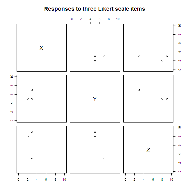
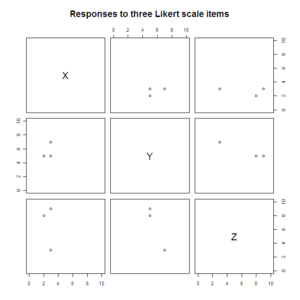
#Scatterplot matrices
pairs(data.3D[2:4], xlim=c(0, 10), ylim=c(0, 10),
main="Responses to three Likert scale items")
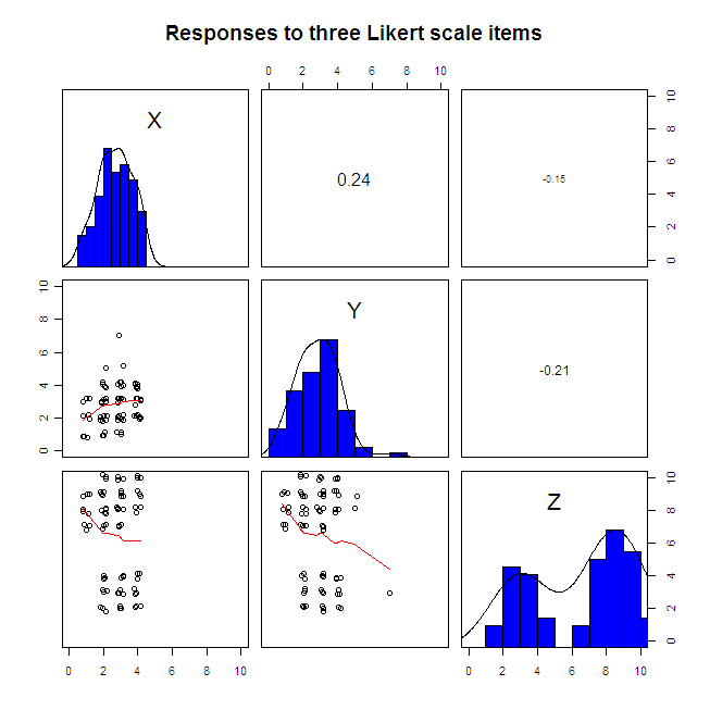
library(psych)
pairs.panels(sapply(data.4D[1:3], jitter), xlim=c(0, 10), ylim=c(0, 10), ellipses=F,
hist.col="blue", pch=1, scale=T, main="Responses to three Likert scale items")

#Load ggplot2 library; set theme without gray background.
library(ggplot2)
theme_set(theme_bw())
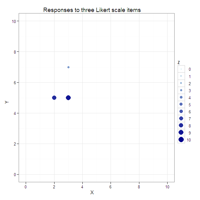
#Create a scatterplot with size and color varying by the third dimension.
plot1 <- ggplot(data=data.3D, aes(x=X, y=Y, color=Z, size=Z)) +
geom_point() +
xlim(0, 10) +
ylim(0, 10) +
scale_colour_gradient(breaks=0:10, limits=c(0, 10), low="lightblue", high="darkblue") +
scale_size_continuous(breaks=0:10, limits=c(0, 10)) +
opts(title="Responses to three Likert scale items")
plot1
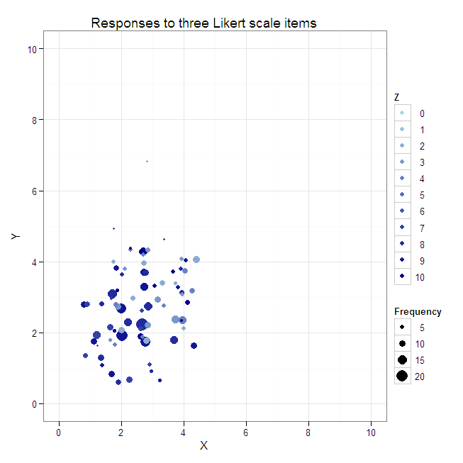
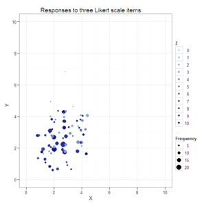
#Create a jittered scatterplot with color varying by the third dimension
#and size by response combination frequency.
plot2 <- ggplot(data=data.4D, aes(x=X, y=Y, color=Z, size=Frequency)) +
geom_jitter() +
xlim(0, 10) +
ylim(0, 10) +
scale_colour_gradient(breaks=0:10, limits=c(0, 10), low="lightblue", high="darkblue") +
scale_size_continuous() +
opts(title="Responses to three Likert scale items")
plot2

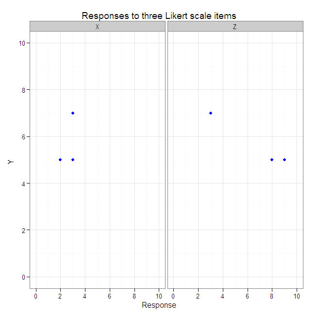
#Reshape data from wide to longer.
data.3D.longer <- melt(data.3D, id.vars=c("Subject", "Y"), variable_name="Item")
names(data.3D.longer)[which(names(data.3D.longer)=="value")] <- "Response"
data.3D.longer
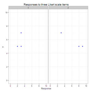
#Create a scatterplot with faceted second and third dimensions.
plot3 <- ggplot(data=data.3D.longer, aes(x=Response, y=Y)) +
geom_point(color="blue") +
xlim(0, 10) +
ylim(0, 10) +
facet_grid(. ~ Item) +
opts(title="Responses to three Likert scale items")
plot3
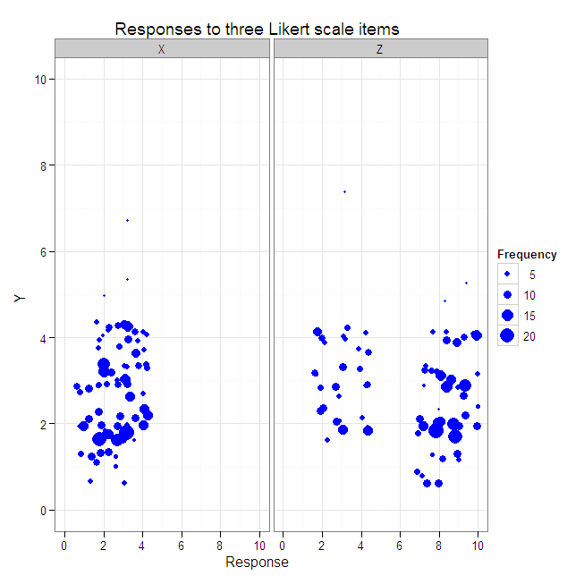
#Reshape simulated data from wide to longer.
data.4D.longer <- melt(data.4D, id.vars=c("Y", "Frequency"), variable_name="Item")
names(data.4D.longer)[which(names(data.4D.longer)=="value")] <- "Response"
head(data.4D.longer)
#Create a scatterplot with faceted second and third dimensions
#and size varying by response combination frequency.
plot4 <- ggplot(data=data.4D.longer, aes(x=Response, y=Y, size=Frequency)) +
geom_jitter(color="blue") +
xlim(0, 10) +
ylim(0, 10) +
facet_grid(. ~ Item) +
opts(title="Responses to three Likert scale items")
plot4