Multilevel Rasch

After years of studying and applying quantitative social science research methods, it has become easier to catch glimpses of larger connections between seemingly independent methodological approaches. I have learned, for example, that survey development has a lot in common with test development. I have also learned that longitudinal data analysis is like spatial/geographic data analysis in that both attend to reference-based dependencies (i.e., one dimensional time and two-or-more dimensional space).

Many methods seem independent because they are taught in isolation as topics courses (e.g., survey methods) or only within disciplines where they are traditionally applied (e.g., social network analysis within sociology). I credit my professors with teaching me to see the larger connections. I also credit the University of Minnesota with offering interdisciplinary courses, such as Latent Variable Measurement Models and Path Analysis taught by Melanie Wall in Biostatistics–a course traditionally taught by psychologists.

Item response theory (IRT) scaling and multilevel modeling are two other quantitative methods that have more in common than they seem at first glance. The Rasch model is usually expressed as

,

where represents a test taker’s latent ability, and represents the difficulty of an item. The Rasch model can also be expressed as a generalized linear model (GLM) with a logit link:

,

where is a dummy variable (1 if a correct response, 0 otherwise) and is the easiness of an item.

Test development designs can be thought of as multistage sampling designs in which test takers represent primary sampling units and item responses represent secondary sampling units nested within test takers. Items can also be thought of as primary sampling units in which responses are nested. If item responses exhibit sizable intraclass correlation, then mixed-effects modeling may be appropriate to account for loss of statistical power relative to simple random sampling. Mixed-effects models may also help with vertical scaling and identifying differential item functioning (DIF) by considering fixed effects for test taker age and group membership. Some authors treat items as fixed effects; while others treat them as random effects. In the latter case, the Rasch model can be expressed as a two-level mixed model with crossed random effects:

.

Posted in Praxes | 2 Comments

Regression discontinuity gallery: R code for nonparametric estimation

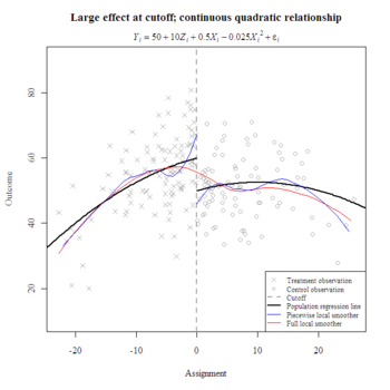
Choosing a functional form for the relationship between the assignment and outcome variable from a regression discontinuity design is an important step in estimating the local average treatment effect. Plotting nonparametric smoothers can suggest a functional form, and nonparametric inference may be more appropriate when a curvilinear relationship defies classification. Some researchers exclusively prefer locally-weighted regression because they feel it objectively and conservatively excludes distal observations, although the choice of bandwidth can be subjective.

The following example shows a way to obtain and plot nonparametric estimates with Rlogo.jpg. The approach yields an effect size estimate of about 2.1 standard deviations, which is over twice as large as the true effect (1 σ) and much worse than the parametric estimates (1.1 SD). Increasing the default span from 0.75 to 1 (not shown) improved the estimate slightly (1.3 SD), as did reducing it to 0.5 (1.6 SD). It would be interesting to conduct a simulation study to compare parametric and nonparametric effect size recovery over many random samples while systematically varying regression functions, bandwidths, and cutoff locations.

#Simulate and plot the data as described in the first part of the previous entry.

#Use the full sample to fit a locally-weighted regression line.
lo <- loess(y ~ x, surface="direct")
x.lo <- min(x):max(x)
pred <- predict(lo, data.frame(x=x.lo))
lines(x.lo, pred, col="red")

#Use treatment observations to fit a locally-weighted regression line.
lo.tx <- loess(y ~ x, data.frame(y, x)[which(x<0),], surface="direct")
x.lo.tx <- 0:min(x)
pred.tx <- predict(lo.tx, data.frame(x=x.lo.tx))
lines(x.lo.tx, pred.tx, col="blue")

#Use control observations to fit a locally-weighted regression line.
lo.c <- loess(y ~ x, data.frame(y, x)[which(x>=0),], surface="direct")
x.lo.c <- 0:max(x)
pred.c <- predict(lo.c, data.frame(x=x.lo.c))
lines(x.lo.c, pred.c, col="blue")

#Add legend.
legend("bottomright", bg="white", cex=.75, pt.cex=.75, c("Treatment observation", "Control observation", "Cutoff", "Population regression line ", "Piecewise local smoother", "Full local smoother"), lty=c(NA, NA, 2, 1, 1, 1), lwd=c(NA, NA, 2, 2, 1, 1), col=c("darkgrey", "darkgrey", "darkgrey", "black", "blue", "red"), pch=c(4, 1, NA, NA, NA, NA))

#Nonparametric estimate [95% confidence interval] of local average treatement effect.
yhat.tx <- predict(lo.tx, 0, se=T)
yhat.c <- predict(lo.c, 0, se=T)
yhat.tx$fit - yhat.c$fit
c((yhat.tx$fit - qt(0.975, yhat.tx$df)*yhat.tx$se.fit) - (yhat.c$fit + qt(0.975, yhat.c$df)*yhat.c$se.fit), (yhat.tx$fit + qt(0.975, yhat.tx$df)*yhat.tx$se.fit) - (yhat.c$fit - qt(0.975, yhat.c$df)*yhat.c$se.fit))

Yields 21.28786 [7.453552, 35.122162].

Local_Effect_Continuous_Quadratic_Relationship_Nonparametric.png

Posted in Praxes | 2 Comments

Regression discontinuity gallery: R code

A reader who is studying political science at the University of Chicago asked me how I plotted the regression discontinuity simulations in my previous blog entry. Here’s a reproducible example for those of you conducting regression discontinuity analyses with Rlogo.jpg:

#Randomly sample from X~N(0, 100) and conveniently use mean cutoff to maximize power and bypass centering.
set.seed(100)
x <- rnorm(200, 0, 10)
z <- ifelse(x<0, 1, 0)
tx <- which(z==1) #Randomly sample from T~N(50, 100) and specify the regression function.
set.seed(101)
y <- rnorm(200, 50, 10) + 10*z + 0.5*x - 0.025*x^2 #1 σ effect size #Plot the observations and regression lines.
plot(y ~ x, col=NULL, xlab="Assignment", ylab="Outcome", ylim=c(min(y)-10, max(y)+10))
abline(v=0, lty=2, lwd=2, col="darkgrey")
points(x[tx], y[tx], col="darkgrey", pch=4)
points(x[-tx], y[-tx], col="darkgrey")
curve(50 + 10 + 0.5*x - 0.025*x^2, min(x)-10, 0, add=T, lwd=2)
curve(50 + 0.5*x - 0.025*x^2, 0, max(x)+10, add=T, lwd=2)
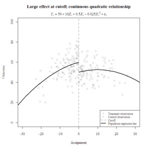
title(main="Large effect at cutoff; continuous quadratic relationshipn")
mtext(expression(italic(Y[i]) == 50 + 10*italic(Z[i]) + 0.5*italic(X[i]) - 0.025*italic(X[i])^2 + italic(epsilon[i])), line=.5)

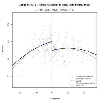
I prefer to plot lines with curve() instead of predict() when the regression equation is simple. The former only requires coefficients and produces nice smooth curves; the latter requires a data frame and may result in jagged lines but is well-suited for lengthy equations with many interactions. Here’s a way to plot fitted lines with parameter estimates from lm():

#Fit a regression discontinuity model.
model <- lm(y ~ z + x + I(x^2))
print(xtable(model), type="html")

Estimate Std. Error t value Pr(&gt |t|)
(Intercept) 49.5272 1.4028 35.31 0.0000
z 11.1037 2.1343 5.20 0.0000
x 0.5231 0.1173 4.46 0.0000
I(x^2) -0.0311 0.0055 -5.67 0.0000

#Add the fitted lines and legend.
coefs <- coefficients(model)
curve(coefs[1] + coefs[2] + coefs[3]*x + coefs[4]*x^2, min(x)-10, 0, add=T, col="blue")
curve(coefs[1] + coefs[3]*x + coefs[4]*x^2, 0, max(x)+10, add=T, col="blue")
legend("bottomright", bg="white", cex=.75, pt.cex=.75, c("Treatment observation ", "Control observation", "Cutoff", "Population regression line ", "Fitted line"), lty=c(NA, NA, 2, 1, 1), lwd=c(NA, NA, 2, 2, 1), col=c("darkgrey", "darkgrey", "darkgrey", "black", "blue"), pch=c(4, 1, NA, NA, NA))

Note the decreasing accuracy of predictions further away from the cutoff, where fewer observations lie.

Local_Effect_Continuous_Quadratic_Relationship_with_Fitted_Line.png

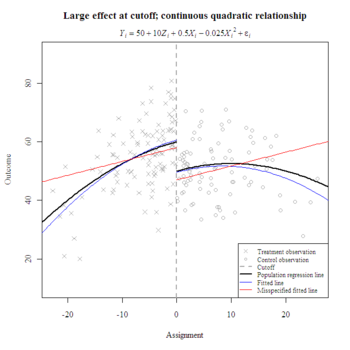
What happens when one misspecifies the functional form? In the following example, the linear misspecification poorly represents the true conditional mean, especially beyond the cutoff. However, the local effect size estimate (i.e., at the cutoff) compares favorably to the estimate from the correct specification. Both have overestimated the true local effect by about one-tenth of a standard deviation.

#Fit a misspecified regression discontinuity model.
model <- lm(y ~ z + x)
print(xtable(model), type="html")

Estimate Std. Error t value Pr(&gt |t|)
(Intercept) 46.9717 1.4296 32.86 0.0000
z 11.0570 2.2969 4.81 0.0000
x 0.4742 0.1259 3.77 0.0002

#Add the fitted lines to the first plot and update the legend.
coefs <- coefficients(model)
curve(coefs[1] + coefs[2] + coefs[3]*x, min(x)-10, 0, add=T, col="red")
curve(coefs[1] + coefs[3]*x, 0, max(x)+10, add=T, col="red")
legend("bottomright", bg="white", cex=.75, pt.cex=.75, c("Treatment observation ", "Control observation", "Cutoff", "Population regression line ", "Fitted line", "Misspecified fitted line"), lty=c(NA, NA, 2, 1, 1, 1), lwd=c(NA, NA, 2, 2, 1, 1), col=c("darkgrey", "darkgrey", "darkgrey", "black", "blue", "red"), pch=c(4, 1, NA, NA, NA, NA))

Local_Effect_Continuous_Quadratic_Relationship_with_Misspecified_Fitted_Line.png

Posted in Praxes | Comments Off on Regression discontinuity gallery: R code

Regression discontinuity gallery: Simulations in R

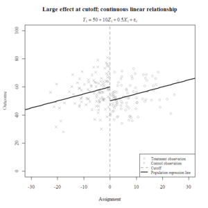
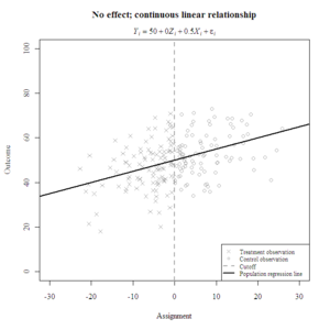
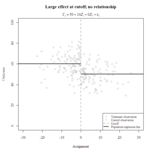
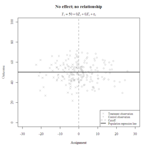
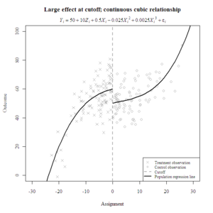
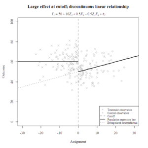
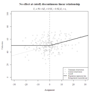
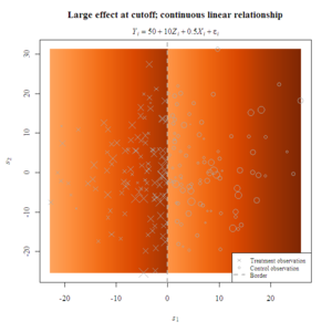
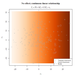
I recently presented a paper on spatial regression discontinuity at the annual conference of the American Evaluation Association in Orlando. I wanted to graphically illustrate regression discontinuity and its spatial analogue, so I simulated some examples in Rlogo.jpg. Plots such as these and William Trochim’s can be a good way to convey some of the key concepts of regression discontinuity design and analysis, such as curvilinear relationships between the assignment and outcome variable, local treatment effects, and the questionable validity of extrapolating program inferences beyond the cutoff.

Local effect (left) and no effect (right) with continuous linear relationship between the assignment and outcome variable
Local_Effect_Continuous_Linear_Relationship.png No_Effect_Continuous_Linear_Relationship.png

Average effect (left) and no effect (right) with no relationship between the assignment and outcome variable
Average_Effect_No_Relationship.png No_Effect_No_Relationship.png

Local effects with curvilinear relationships between the assignment and outcome variable
Local_Effect_Continuous_Quadratic_Relationship.png Local_Effect_Continuous_Cubic_Relationship.png

Extrapolation: Local effect (left) and no local effect (right) with potentially larger effects beyond the cutoff due to discontinuous linear relationship between the assignment and outcome variable*
Local_Effect_Discontinuous_Linear_Relationship.png No_Effect_Discontinuous_Linear_Relationship.png
*Note: Extrapolations beyond the cutoff are rarely valid. Repetitious and abundant distal pretest observations may support extrapolating effect size estimates beyond the cutoff.

Spatial regression discontinuity: Local effect (left) and no effect (right) with continuous linear relationship between the assignment (distance from border) and outcome variable
Local_Effect_Continuous_Linear_SpatialRD.png No_Effect_Continuous_Linear_Relationship_SpatialRD.png

Posted in Praxes | Comments Off on Regression discontinuity gallery: Simulations in R

Urban canoeing: Minneapolis to Saint Paul

IMG_0503.jpg IMG_0502.jpg

Sometimes I enjoy seeing architecture and other human artifacts from the river’s vantage point as much as I like experiencing nature. Garbage and pollution are major exceptions.

The Mississippi River offers a great mix of nature and civilization as it flows through Minneapolis toward Saint Paul: bald eagles flying near skyscrapers, blue herons fishing from the dams, geese wading under bridges, and trees clinging to public beaches.

IMG_0493.jpg

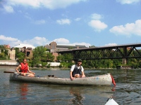
My friend, Chris Desjardins, a veteran of the Mississippi River Challenge, guided us down the urban route from Boom Island Park to Hidden Falls Park. The photo at right shows us paddling past the Education Sciences Building where our offices are located.

We hoped to make it to the backwaters near the Minnesota River confluence, but it took too long to navigate the locks with so many boats on the river for Labor Day. I plan on putting in at Hidden Falls for my next urban trip.

Posted in Personal | Comments Off on Urban canoeing: Minneapolis to Saint Paul